This article is published as a part of the Data Science Blogathon.
Introduction
In this article, we will go on to discuss the important crux interview question on “Data Science” & “Machine Learning” which is helpful to get a clear understanding of the techniques, and also for Machine Learning, Artificial Intelligence, and Data Science Interviews.
We Believe that you have learned both theoretical and practical knowledge of supervised and unsupervised algorithms.
So let’s test your knowledge here.
Interview Questions
1. Difference between Supervised Learning and Unsupervised Learning.
|
|
| Supervised Learning Algorithms are trained using labeled data(Target Columns). | Unsupervised Learning algorithms are trained by using unlabeled data. |
| The Supervised Learning algorithm aims to train the model to predict the output when given new data. | The Unsupervised Learning algorithm aims to find the hidden patterns and useful insights from the unknown dataset |
| Input data are provided to the model along with the output. | Only input data is provided to the model. |
| Supervised Learning can be categorized in: 1. Classification and 2. Association Problems. |
Unsupervised Learning can be classified in: 1. Clustering and 2. Association Problem. |
2. What is Linear Regression?
Linear Regression establishes a relationship between a dependent variable (Y) and one or more independent variables (X) by finding the best fit of the straight line.
The equation for the Linear model is Y = mX+C,
where m is the slope and C is the intercept.
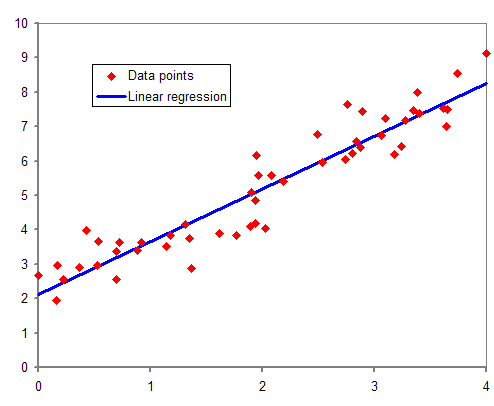
In the above diagram, the red dots we see are the distribution of “Y” concerning X. In the real-life scenario, no straight line runs through all the data points. So, the objective here is to fit the best fit of the straight line that will true to minimize the error between the expected and actual values.
Regression Metrics
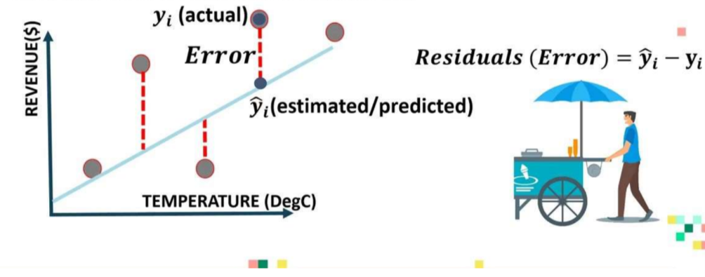
Regression Metrics:

3. Explains the Errors in the Regression Model:
1. Mean Absolute Error (MAE):
MAE is calculated by calculating the absolute difference between the model Predictions and True (actual) values.
MAE is a measure of the average magnitude of error generated by the regression model:

If MAE is zero, this indicates that the model predictions are perfect.
2. Mean Square Error (MSE):
MSE is very Similar to the mean absolute error (MAE). In MAE instead of using Absolute values, squares of the difference between the model predictions and the training dataset (True values) are calculated.
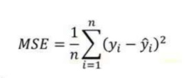
MSE values are generally larger than MAE since the residuals are squared. In the case of data outliers, MSE will become much large compared to MAE.
In MSE, since the error is squared, any predicting error is heavily penalized.
3. Root Mean Square Error (RMSE) :
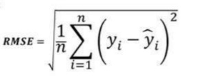
Root Mean Square Error (RMSE) represents the standard deviation of residues (the difference between model predictions and true values (training data).
RMSE provides an estimate of the size of the dispersed residue.
RMSE can be easily translated compared to MSE because RMSE units are similar to output units.
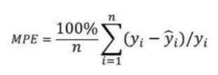
4. Mean Percentage Error (MPE):
Mean Percentage Error (MPE) is useful to provide an insight into how many positive errors as compared to the negative ones.
5. Mean Absolute Percentage Error (MAPE):
Mean absolute error values can range from zero to infinity, making it difficult to interpret the result compared to training data.
Mean absolute percentage error is the equivalent to MAE but provides the error in the percentage form and therefore overcomes the MAE limitations.
MAPE might exhibit some limitations if the data point value is zero( since there is the division operator involved).

4. What is R-Square and What Exactly is R-Square Represents?
1. R-Square represents the proportion of variances of the dependent variable (Y) that has been explained by the independent variables.
2. R-Square Provides insight into the Goodness of fit.
3. The maximum R-Square value is 1.
4. Consistent model that always predicts the expected value of y ignoring the input features will have an R-Square rating of 0.

5. What is the difference between R-Square and Adjusted R-Square?
R-Square ( R² ) explains the degree to which your input variables explain the variation of your output/predicted variable.
If R-Square is 0.8 means 80% of the variation in the output is explained by input variables. So in simple, the Higher the R-Squared, the more variation is explained by your input variables, and hence better is our model.
One of the limitations of the R-Square is that it increases by adding independent variables to the model even if they do not have any relationship with the output variable or a very minimal relationship with output variables.
This is where Adjusted R-square comes to help. Adjusted R-Square overcomes this issue by adding a penalty if we attempt to add an independent variable that does not improve the model.
If useless predictors are added to the model, adjusted R-Square will decrease.
If useful predictors are added to the model, adjusted R-Square will increase.

alphabet k denotes the number of independent variables and alphabet n denotes the number of samples.
Hence, if you are developing a Linear Regression model on multiple variables. It is always suggested that you use an adjusted R-Squared to judge the goodness of the model. In case you have only one input variable R-Square and Adjusted R-Square would be the Same.
6. What are the Assumptions in the Linear Regression?
Linear regression is a statistical model that allows to explains of a dependent variable y based on variation in one or multiple independent variables (denoted X). It does this based on the linear relationship between the dependent and independent variables.
1. Linearity / Linear Relationship: there is a linear relationship between the independent variable X and the dependent variable Y. The easiest way to detect if this assumption is met is to create a scatter plot of X versus Y. This allows you to visualize if there is a linear relationship between these two variables.
2. Independence: The Next assumption of the Linear regression is that the residuals are independent. It is most relevant when working with time-series data. Ideally, we do not want there to be a pattern between successive remnants. The simplest way to test if this assumption is met is to look at the residual time series plot, which is a plot of residuals versus time.
3. Normality: The Next Assumption of Linear Regression is that the residuals are “Normally distributed”. A Q-Q plot, short for quantile plot, is a type of plot that we can use to determine whether or not the residuals of a model follow a normal distribution. If the points on the graph roughly form a straight diagonal line, then the normality assumptions are met.
4. Equal Variance / Homoscedasticity: Residuals have constant variance at every Level of X (independent variable). It is known as Homoscedasticity. Once you fit a regression line to a set of data, you can then create a scatterplot that shows the fitted values of the model versus the residuals of those Fitted values.
7. What is the difference Between Regression and Correlation?
Correlation: In the real scenario, correlation measures the strength or degree of relationship between two variables. It does not capture causality. “Correlation” express by a single point.
Regression: Measures how one variable affects another variable. “Regression” is about model fitting. It tries to capture causality and explain the cause and effect. “Regression” express by a regression line.
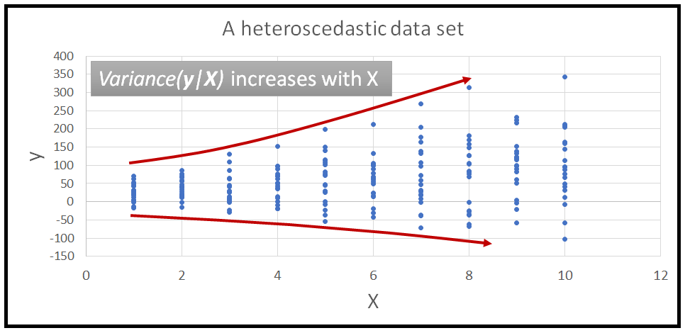
8. What is Heteroscedasticity? How to detect it?
Heteroscedasticity refers to the situation where the variance of the residuals is unequal over a range of measured values. When running a regression analysis, “Heteroscedasticity” results in an unequal scatter of the residuals (also known as the error term).
9. What is an intercept in a Linear Regression? What is its significance?
The intercept is the point at which the function crosses the Y-axis. An intercept is a standard mean value of Y value when all X = 0.
10. What is OLS?
OLS stands for Ordinary Least Square. The main objective of the Linear Regression algorithm is to find the coefficients or estimates by minimizing the error terms such that the sum of squared error should be minimum. This process is known as OLS.
This method finds the best fit line, known as the Regression Line, by minimizing the sum of the difference of the squares between the observed and predicted values.
11. What is Multicollinearity?
Reasons for Multicollinearity:
1. Inaccurate use of dummies.
2. Due to variables that can be computed from another variable in the dataset.
Detecting Multicollinearity:
1. By using the Correlation Coefficient.
2. With the help of variance inflation factor (VIF) and Eigenvalues.
12. What is VIF? How do you calculate it?
VIF Stands for variance inflation factor, which determines how much variance of an estimated regression coefficient increased due to the presence of collinearity between the variables. It also calculates how much multicollinearity is present in a particular regression model.
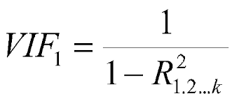
It is always desirable to have the VIF value as low as possible. A threshold is set, Which means that any independent variable larger than the threshold will have to remove.
13. For a Linear Regression Model, How do we interpret a Q-Q plot?
The Q-Q plot is used to represent a graphical plotting of the quantile of two distributions concerning each other. In simple words, the Q-Q plot is used to check the normality of errors.
Whenever we interpret a Q-Q plot, we should concentrate on the y=x line, which corresponds to a normal distribution. Sometimes this is also known as the 45-degree line in Statistics.
Usage of Q-Q plot:
1. Check whether two samples are from the same population.
2. Whether two samples have the same tail.
3. Whether two samples have the same distribution shape.
14. Why Absolute error is preferred instead of squared error?
1. The absolute error is often closer to what we want when making predictions from our model. But if we want to penalize those predictions that are contributing to the maximum values of error.
2. in the Mathematical terms, the squared function is differentiable everywhere, while the absolute error is not differentiable at all the points its derivative is undefined at 0. It makes the squared error more preferable to the techniques of mathematical optimization.
3. we use the root mean squared error instead of the mean squared error so that the unit of RMSE and the dependent variable are equal and the results are interpretable.
15. What are the disadvantages of Linear Regression algorithms?
1. Assumption of Linearity: it always assumes that there exists a linear relationship between the independent variables (input) and dependent variable (output). Therefore we are not able to fit the complex problem with the help of linear Regression.
2. Outliers: it is highly sensitive to outliers.
3. Multicollinearity: it gets affected by the Multicollinearity.
16. What is Regularization? Explain its Types?
Regularization aims to solve a number of common model problems by:
1. Minimizing model complexity.
2. Penalizing the loss function.
3. Reducing model overfitting (add more bias to reduce model variance).
In general, we can generally explain that regularization is a way to reduce model-Overfitting and variance. For this-
1. It Requires some additional bias
2. Requires a search for optimal penalty hyperparameter.
types:
1. L2 Regularization: Ridge Regression
2. L1 Regularization: LASSO Regression
3. Combining L1 and L2: Elastic Net
L2 Regularization: Ridge Regression
Ridge Regression works by applying a penalizing term( Reducing the weight and biases) to overcome overfitting.
In Ridge, the Regression slope has reduced with the ridge regression penalty term, so the model becomes less sensitive to changes in the independent variables.
Least Square Regression: Min(sum of squared residuals)
Ridge Regression : Min(sum of the squared Residuals + α .(Slope)²)
L1 Regularization: LASSO Regression
Lasso Regression is similar to ridge regression. It works by introducing a bias term but instead of Squaring the Slope, the absolute( Modulus) value of the slope is added as a “penalty term”.
Least Square Regression: Min(sum of squared residuals)
Ridge Regression : Min(sum of the squared Residuals + α |Slope|)
Elastic Net:
Elastic Net is a popular type of regularized Linear Regression that combines Both L1 and L2 Penalty terms.
17. What is the Classification algorithm in Machine Learning?
The classification algorithm is a supervised learning technique used to identify the Category of new observation based on the training data. In classification, a program learns from the given dataset or the observations and then classifies new observations into several classes or groups such as YES or NO. 0 or 1. Spam or Not Spam. Classes can be called targets or Categories.
1. Binary classifier: if the Classification problem has only two possible outcomes, then it is called a Binary Classifier.
Example: Yes or NO, Male or Female, Spam or Not Spam
2. Multiclass Classifier: If the problem has more than two outcomes, then it is known as a Multiclass Classifier.
Example Classification of types of crops, Classification of types of music.
Classification algorithms can be further divided into the main two categories:
1. Linear Models:
1. Logistic Regression
2. Support Vector Machines.
2. Non-Linear Models:
1. K-Nearest Neighbors
2. Kernel SVM
3. Naive Bayes
4. Decision tree Classification
5. Random Forest Classification.
18. What do you understand by Confusion Matrix? Explain?
2. Confusion Matrix compares the actual target values with the predicted values with the help of a machine learning model.
3. Also known as the error matrix.
19. What is the AUC-ROC curve?
1. ROC Curve stands for Receiver Operating Characteristics Curve & AUC stands for Area Under the Curve.
2. It is the graph that shows the performance of the classification model at different thresholds.
3. For visualization of the performance of the multiclass classification model, we use the AUC-ROC curve.
4. The ROC curve is plotted with FPR (False Positive Rate) on X-axis and TPR (True Positive Rate) on Y-axis.
5. If ROC-AUC = 1, Perfect classifier.
20. What is Logistic Regression?
Logistic regression is s Supervised Learning classification algorithm used to predict the probability of the target variable.
The nature of the target or dependent is inseparable, which means that there will be only two possible categories.
In simple words, The dependent variable is Binary in Nature having data coded as either 1 or 0.
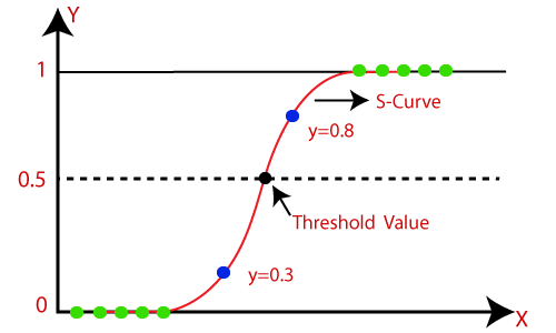
In Logistic Regression, instead of fitting a regression line, we fit an “S” shaped logistic function, Which predicts two maximum values ( 0 or 1 ).
Example:
1. Whether the Cells are Cancerous or NOT.
2. Students will PASS or FAIL.
21. What is Logistic Function or Sigmoid Function?
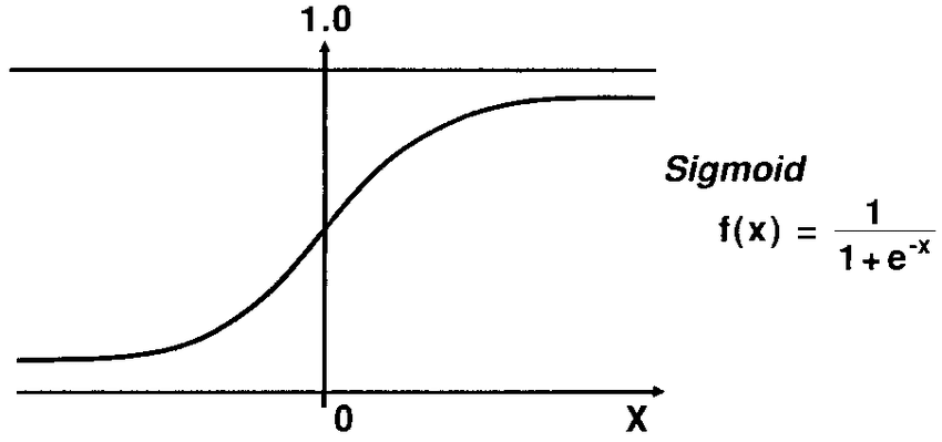
The Sigmoid Function is a Mathematical Function used to Map the Predicted values to the Probability of 0 and 1.
Linear Regression model Generate Predicted values as any number ranging from negative to positive infinity. But we know that probability can be between 0 and 1.
To overcome this problem we use a regression curve, which converts a straight line of a curve into an S-curve using the Sigmoid function, which will always give values between 0 and 1. The S-form curve is called a sigmoid or Logistic function. function.
22. Explain Assumptions in Logistic Regression:
1. There is no or minimum multicollinearity among the independent variables such that predictors are not correlated.
2. There should be a Linear Relation Ship between the Logit of the outcome and each Predictor variable.
3. Usually large sample size is required.
4. It assumes no dependency Between the Observations.
23. Comparison between Linear Regression and Logistic Regression.
| Linear Regression | Logistic Regression |
| Linear Regression is used to predict the continuous dependent variable using a given set of independent variables. | Logistic regression is used to predict the Categorical dependent variable in the form of 0 and 1 using a given set of the independent variable. |
| It is Based on Least Square Estimation Method. | It is based on the Maximum Likelihood Estimation method |
| Here no threshold value is needed. | Here threshold value is needed. |
| In a Linear Regression, it is required that the relationship between a dependent variable and the independent variable must be linear. | It is not required to have a linear relationship between the dependent and Independent variables. |
| In linear regression, there will be the possibility of collinearity between the independent variables. | In Logistic regression, there should be no collinearity between the independent variable. |
Conclusion to Interview Questions
Thank you for reading. I hope you feel confident about appearing in the Data Science interviews. I hope you enjoyed the interview questions and were able to test your knowledge about Data Science and Machine Learning. If you have any feedback or would like to share your views on these comments then please share in the comment box below.
Please feel free to contact me on Linkedin.
email: anurag8200@gmail.com
The media shown in this article is not owned by Analytics Vidhya and is used at the Author’s discretion.


