
Introduction to Predictive Analytics
DonorsChoose.org is an online charity platform where thousands of teachers may submit requests through the online portals for materials and particular equipment to ensure that all kids have equal educational chances. The project is based on a Kaggle Competition for Predicting Excitement at DonorsChoose.org, It looks for initiatives that are both noteworthy and successful.
DonorsChoose is a platform that uses crowdsourcing to close the education funding gap. Since 2000, they have helped 40 million students in the United States receive $970 million in donations. However, around a third of all projects on DonorsChoose are not able to complete the target within four months of their first posting. By ensuring that more projects meet their fundraising targets, this project will aid DonorsChoose in closing the education funding gap. We’ll build an early warning system that detects recently posted projects that are likely to fall short of their financial targets, allowing DonorsChoose to intervene with a donation matching award.DonorsChoose is a publicly available dataset that provides information about teacher-proposed school projects in the US. By using machine learning models to determine donors’ behavior and filter the important projects from the dataset, the suggestion would address the challenge of keeping existing contributors.
You can download the dataset from Kaggle, here is the link.
Architecture
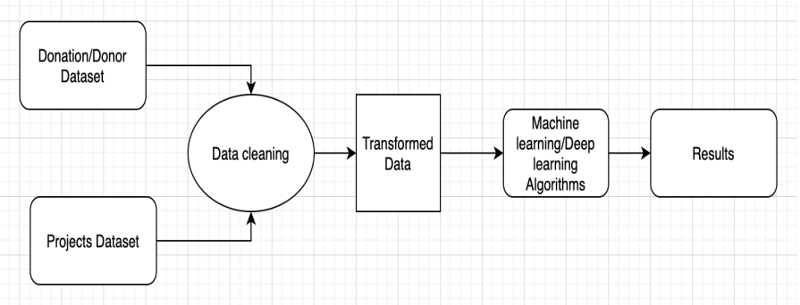
I have focused heavily on the topic of Text Pre-Processing. I would like to summarize all the important steps in one post. Here I will not go into the theoretical background. For that, please read my earlier posts, where I explained in detail what I did and why. Refer
Objective for Predictive Analytics
The objective of the competition is to implement different ML algorithms on the DonorsChoose Dataset and calculate/analyze the accuracy of the Test dataset.
Importing all the necessary libraries to perform the analysis.
 Naive Bayes Classifier
1. Gaussian Naive Bayes
Gaussian naïve Bayes Classifier is maybe the most uncomplicated naive Bayes classifier to grasp. We believe these values are sampled from a Gaussian distribution when the predictors take up a continuous value and are not discrete.
2. Multinomial Naive Bayes
Multinomial Naive Bayes is an NLP-based technique that determines the likelihood of each tag for a certain sample and produces the tag with the highest likelihood. The assumption that Gaussian is the single, obvious assumption that is used for generative distribution. Multinomial naive Bayes is another helpful example, in which the features are believed to be generated by a simple multinomial distribution. Multinomial naive Bayes is best for features that represent counts or count rates since the multinomial distribution describes the chance of detecting counts or repetitive words among a number of categories however, instead of modelling the data distribution with the best-fit Gaussian, we model it with the best-fit multinomial distribution.
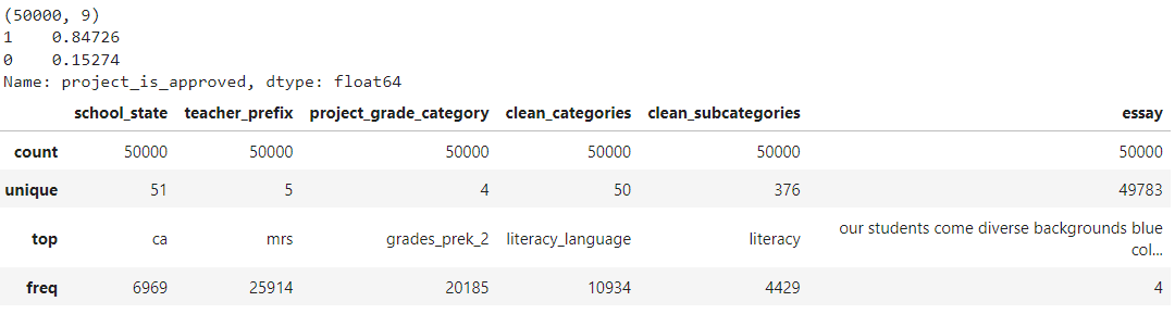
Loading the Data
data = pandas.read_csv('preprocessed_data-Copy1.csv')
print(data.shape)
print(data["project_is_approved"].value_counts(normalize=True))
data.describe(include=["object", "bool"])
Splitting data into Train and Test: Stratified Sampling
y = data['project_is_approved'].values
print(y)
X = data.drop(['project_is_approved'], axis=1)#droping the Y value as we want to predict the output
X.shape
X_train, X_test, y_train, y_test = train_test_split(X, y, test_size=0.33, stratify=y,random_state=42)
Encode the text features i.e. Essay or Project title
BOW
-
We will use this function to discover all unique words in the data and give a dimension-number to each one.
-
If you have a review that says __’ very horrible pizza,’__ you may express each unique phrase with a measurement number like this: dict =’ very’: 1, ‘bad’: 2, ‘pizza’: 3.
-
We’ll build a python dictionary to store all of the unique words, with the key representing the unique phrase and the associated value being the dimension-number.
vectorizer = CountVectorizer(min_df=10,ngram_range=(1,4), max_features=7000)
text_bow = vectorizer.fit(X_train['essay'].values)
print(text_bow.get_feature_names())
X_train_essay = vectorizer.transform(X_train['essay'].values)
X_test_essay = vectorizer.transform(X_test['essay'].values)
TFIDF
What does the abbreviation TF-IDF mean?
-
The TF-IDF weight is a popular weight in text mining and information retrieval. Term frequency-inverse document frequency is known as Term Frequency and Inverse Document Frequency(TF-IDF).
-
This action is used to determine the importance of a word in a group or corpus of texts. The importance of a word increases directly related to its number of appearances in the text, although this is counterbalanced by its frequency in the corpus.
-
Variations of the TF-IDF weighting techniques are often used by search engines to score and rate a document’s relevance in response to a user query. One of the most used strategies is to add the TF-IDF for each query phrase; There are much more intricate ranking algorithms.
tfidf_vector = TfidfVectorizer(min_df=10,max_features=7000)
Text = tfidf_vector.fit(X_train['essay'].values)
print(Text.get_feature_names())
X_train_essay_TFIDF = tfidf_vector.transform(X_train['essay'].values)
X_test_essay_TFIDF = tfidf_vector.transform(X_test['essay'].values)
print(X_train_essay_TFIDF.shape, y_train.shape)
print(X_test_essay_TFIDF.shape, y_train.shape)
Encode the categorical and numerical features
vectorizer_state = CountVectorizer()
vectorizer_state.fit(X_train['school_state'].values)# fit has to happen only on train data
X_train_state = vectorizer_state.transform(X_train['school_state'].values)
X_test_state = vectorizer_state.transform(X_test['school_state'].values)
X_train_price = normalizer.fit_transform(X_train['price'].values.reshape(1,-1))
X_test_price = normalizer.fit_transform(X_test['price'].values.reshape(1,-1))
X_train_price =X_train_price.reshape(-1,1)
X_test_price =X_test_price.reshape(-1,1)
normalizer.fit(X_train['price'].values.reshape(1,-1)) #fitting
Concatenating all the features
from scipy.sparse import hstack
X_tr = hstack((X_train_essay,'All encoded features')).tocsr()
X_te = hstack((X_test_essay,'All encoded features')).tocsr()
Applying Naive Bayes
naive_bayes_1 =MultinomialNB(class_prior=[0.5,0.5])
parameter_1 ={'alpha': list(np.arange(0.001,100,2))}
print(parameter_1)
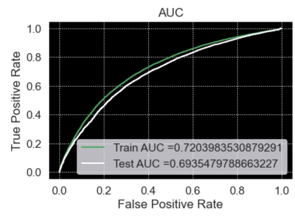
classifier_1 = GridSearchCV(naive_bayes_1,parameter_1,scoring='roc_auc',cv=10,return_train_score=True)
classifier_1.fit(X_tr,y_train)
train_auc_1= classifier_1.cv_results_['mean_train_score']
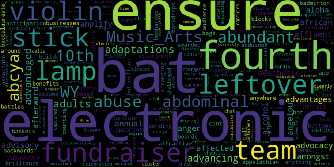
Word Cloud
A word cloud is a text data visualization approach in which the most commonly used term is shown in the largest font size. We’ll learn how to make a custom word cloud in Python in this post.
from wordcloud import WordCloud
from wordcloud import STOPWORDS
#convert list to string and generate
words_string=(" ").join(fp_words)
wordcloud = WordCloud(width = 1000, height = 500).generate(words_string)
plt.figure(figsize=(25,10))
plt.imshow(wordcloud)
plt.axis("off")
plt.show()
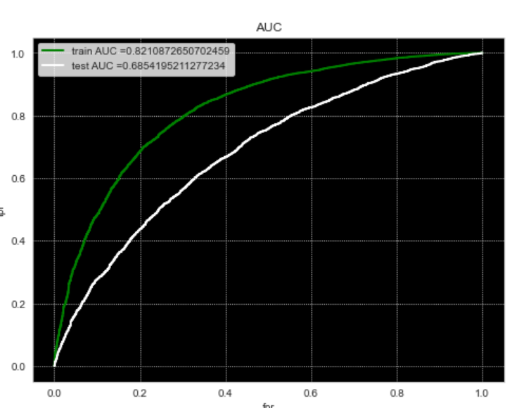
Decision Tree classifier
Difficulties involving categorization and regression, a decision tree is a widely used non-parametric effective machine learning modeling tool. The data is classified using decision trees and is explored in length in the following sections.
To split a node, decision tree algorithms leverage information gain. The criterion for determining information gain is the Gini index or entropy.
Gini and entropy are both the dimensions of a node’s impurity. A node with only one class is pure, as opposed to a node with several classes. The Gini measurement is the likelihood of a random sample being erroneously classified if a label is randomly selected based on the distribution in a branch. Information is measured by entropy. A split is used to compute the information gained.
All the preprocessing part is the same for all models but we’re applying different models to check which model performs well in this dataset. Let’s apply the Decision tree to the preprocessed data.Before that let’s calculate sentiment scores.
import nltk

from nltk.sentiment.vader import SentimentIntensityAnalyzer

sid = SentimentIntensityAnalyzer()

sample_sentence_1='I am happy.'

ss_1 = sid.polarity_scores(sample_sentence_1)

print('sentiment score for sentence 1',ss_1)
Output : sentiment score for sentence 1 {‘neg’: 0.0, ‘neu’: 0.213, ‘pos’: 0.787, ‘compound’: 0.5719}
param_grid= {"max_depth": [1,5,10,50],"min_samples_split": [5,10,100,500]}
model = DecisionTreeClassifier()
clf = GridSearchCV(model,param_grid, cv=3, scoring='roc_auc',return_train_score=True)
clf.fit(X_train1, y_train)
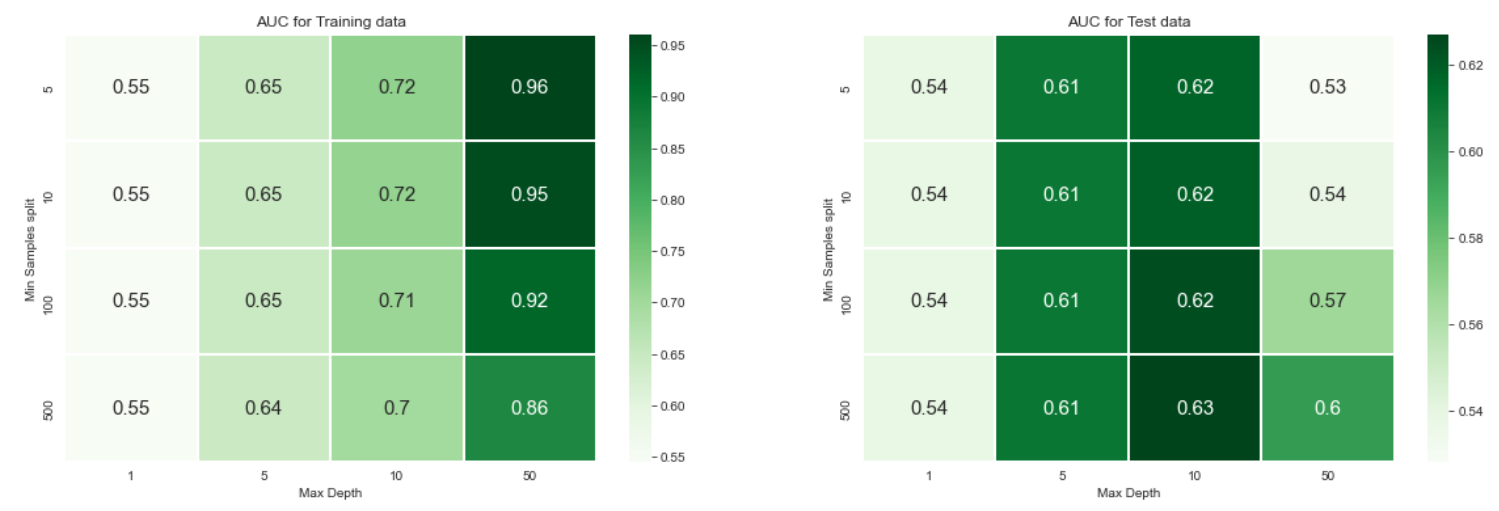
You can refer to this link to know more about the heatmap and confusion matrix.
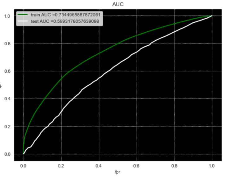
Gradient-boosting Decision Tree (GBDT)
Gradient-boosting differs from AdaBoost in that instead of applying weights to specific samples, GBDT will fit a decision tree based on the preceding tree’s residuals error (thus the name “gradient”). As a result, instead of learning by predicting the target directly, each new tree in the ensemble predicts the prior learner’s inaccuracy.
All the preprocessing part is the same for all models but we’re applying different models to check which model performs well in this dataset. Let’s apply the Decision tree to the preprocessed data.Before that let’s calculate sentiment scores.
from sklearn.ensemble import GradientBoostingClassifier
from sklearn.model_selection import GridSearchCV
parameters = {"max_depth":[1,2,3,4],"min_samples_split":[5,10,15,20] }
clf = GridSearchCV(GradientBoostingClassifier(), parameters, cv=5, scoring='roc_auc',return_train_score=True,n_jobs=-1)
clf.fit(X_train1,y_train)
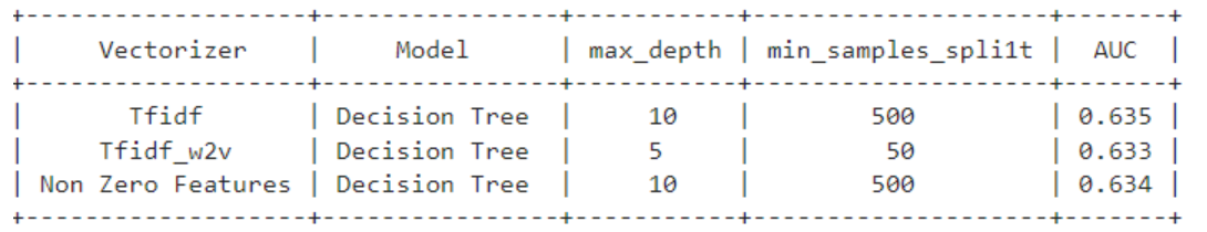
Conclusion to Predictive Analytics
To summarize the data from different models we can use pretty-table for example:
from prettytable import PrettyTable
pretty_table = PrettyTable()
pretty_table.field_names = ["Vectorizer","Model","max_depth","min_samples_spli1t","AUC"]
pretty_table.add_row(["Tfidf","classifier_name ","4","20","0.68"])
pretty_table.add_row(["Tfidf_w2v","classifier_name  ","10","500","0.59"])
print(pretty_table)
- We evaluate each using machine learning techniques aspect of the DonorsChoose dataset in this research.
- Donors approve projects with a high level of project description, according to our findings, because it shows that the essays have an important effect on the AUC score.
- From the analysis, we can clearly see that the project resource summary and DateTime had a positive outcome, indicating that projects that are budget-friendly and provide a clear explanation of how utilities should be used are important.
- Important terms like a workbook, assistant, and classwork were chosen as high likelihood values in both negative and positive classes so using the Naive Bayes technique we can see the probability score for each word. When dealing with textual data, distance-based algorithms suffer from the curse of dimensionality, and training neural networks appears to be more promising.
The media shown in this article is not owned by Analytics Vidhya and is used at the Author’s discretion.
Hello Shradhanjali Pradhan! It's great to meet you. As a working professional and an AI/ML engineer, you must have a strong foundation in data science. Your knowledge and skills in this field are undoubtedly invaluable to any organization that values data-driven decision-making. I'm excited to hear more about your experiences and insights in the field, and I'm here to assist you in any way I can. Let me know if you have any questions or if there's anything I can help you with.


