What are Schemas in Data Warehouse Modeling?

This article was published as a part of the Data Science Blogathon.

Introduction

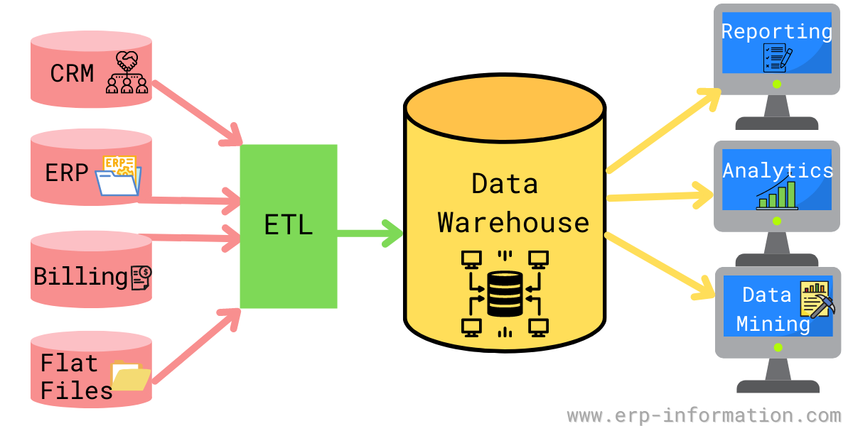
Do you think you can derive insights from raw data? It’s possible, of course, but it can be tiresome and not be as accurate as it should be. Wouldn’t the process be much easier if the raw data were more organized and clean? Here’s when Data warehousing comes in handy. It is the process of constructing a data warehouse containing essential data. We need to archive and store the data for future use. ETL (Extract, Transform and Load) turns raw data into information. Through this article, let’s understand schemas and their role in data warehouse modeling.

Data Warehouse

A Data warehouse is a digital location to store data from many sources such as databases and files. To solve a business question and make data-driven decisions, we need to mine the data. We do this through this central data repository to get insights and generate reports. It works based on OLAP (Online Analytical Processing). As a result, it is a location to store an organization’s historical and archived data. It is also the single source of truth. All the required information (organized data) is present in a single place. It helps to answer a detailed-oriented question and find trends in historical data.

Image Source

Data Modeling

Before building a building, we first need to create its design and make a model. In the same way, to create a data warehouse, we need to design it first using data warehouse modeling tools and techniques. We do this to represent the data in the real world and see how business concepts relate. Data warehouse modeling is the process of designing the summarized information into a schema.

Schema

Schema means the logical description of the entire database. It gives us a brief idea about the link between different database tables through keys and values. A data warehouse also has a schema like that of a database. In database modeling, we use the relational model schema. Whereas in the data warehouse, we use modeling Star, Snowflake, and Galaxy schema.

To get a good understanding of how a Schema looks. Let’s look at an example Schema of the top_terms table. It is from the google_trends database in Google BigQuery.

Key Concepts of Schemas

Image Source

1. Primary Key – An attribute in a relational database having unique values. There are no duplicate values. We identify each record with its unique value. In the above example, Stud_id is the primary key. It is because each student will have only one unique id.

2. Foreign Key – An attribute in a relational database that links one table to another. It refers to the primary key from another table. In the above example, Stud_id is the foreign key in the department table. It is because it was the primary key in the student table. We link the student and the department table together via joins.

3. Dimensions – Dimensions are the column names in a dimension table. Also, dimensions have their attributes sub-divided in the table. We use dimensions as a structured way of describing and labelling the information. Dimension tables are the tables describing dimensions. Example: Date, products, and customers are some common dimensions.

4. Measures – Quantitative attributes in the fact table. We perform calculations like average and sum on them. Example: No. of products, discount.

5. Fact Table – A fact table contains a dimension key from the dimension table and measures. The measures here are to perform calculations for analysis. The dimension key and measures describe the facts of the business processes. A fact table consists of measurements of our interests. Example: Product_id, Date_id, No. of products.

Schema Definition

Data Mining Query Language (DMQL) defines Multidimensional Schema. Using a multidimensional schema, we model data warehouse systems. Cube definition and dimension definition are the two primitives. This is because we view data in the form of a data cube. They help to define data warehouses and data marts.

CUBE DEFINITION

SYNTAX

define cube  []:

DIMENSION DEFINITION

SYNTAX

define dimension  as ()

Types of Schemas

There are three main types of data warehouse schemas :

1. Star Schema

2. Snowflake Schema

3. Galaxy Schema

Star Schema

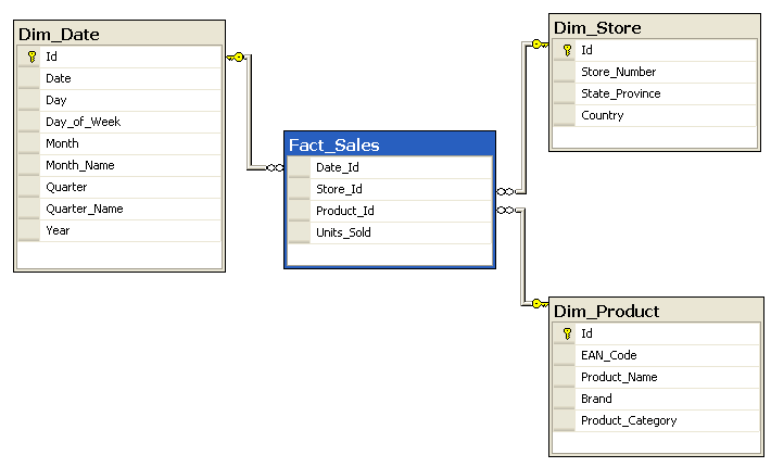
Star Schema is the easiest schema. It has a fact table at its centre linked to dimension tables having attributes. It is also called as Star-Join Schema. It has a primary and foreign key relationship between the dimension table and the fact table. It is de-normalized means the normalization is not done as it is for relational databases. Its characteristic is that we represent each dimension with only a one-dimension table. Example: The Fact_Sales table has Date_id, Store_id, and Product_id as the dimension keys. These keys link to only one dimension table per key.

In the diagram below, Fact_Sales is the fact table. Dim_Date, Dim_Store, and Dim_Product are the dimension tables. Id, Store_Number, State_Province, and Country are the attributes of the dimension table Dim_Store. In the same way, other dimension tables have their attributes.

ADVANTAGES: 

1. Most Suitable for Query Processing: View-only reporting applications show enhanced performance.

2. Simple Queries: Optimized Navigation through the database. It is because the star-join schema logic is much simpler.

3. Simplest and Easiest to design.

DISADVANTAGES:

1. They don’t support many to many relationships between business entities.

2. More data redundancy: It is a result of each dimension having only one dimension table.

DEFINING A STAR SCHEMA IN DMQL FOR THE DIAGRAM BELOW

define cube Fact_Sales_star [Dim_Date, Dim_Store, Dim_Product]:Units_Sold = count(*)

define dimension Dim_Date as (Date_Id, Date, Day, Day_of_Week, Month, Month_Name, Quarter, Quarter_Name, Year)

define dimension Dim_Store as (Store_Id, Store_Number, State_Province, Country)

define dimension Dim_Product as (Product_Id, EAN_Code, Product_Name, Brand, Product_Category)

Image Source

Snowflake Schema

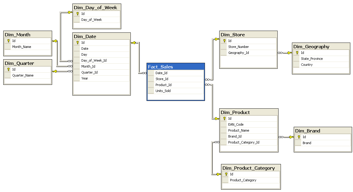
It is an extended version of the star schema where dimension tables are sub-divided further. It means that there are many levels of dimension tables. It is because of the normalized dimensions here. Normalization is a process that splits up data to avoid data redundancy. This process sub-divides the tables and the number of tables increases. The Snowflake schema is nothing but a normalized Star schema.

The following diagram shows Dim_Store has Id, Store_Number, and Geography_Id as its attributes. There is a link between Geography_Id and the Dim_Geography dimension table. The Dim_Geography dimension table has Id, State_Province, and Country as its attributes. In the same way, Dim_Date and Dim_Product are normalized.

ADVANTAGES:

1. Easy to maintain: It is due to reduced data redundancy.

2. Saves Storage space: Dimension tables are easier to update.

DISADVANTAGES:

1. Complex Schema: Source query joins are complex.

2. Query Performance is not so good: because of the complex queries.

DEFINING A STAR SCHEMA IN DMQL FOR THE DIAGRAM BELOW

define cube Fact_Sales_snowflake [Dim_Date, Dim_Store, Dim_Product]:Units_Sold = count(*)

define dimension Dim_Date as (
        Date_Id, Date, Day,
        Dim_Day_of_Week (Day_of_Week_Id, Day_of_Week),
        Dim_Month (Month_Id, Month_Name),
        Dim_Quarter (Quarter_Id, Quarter_Name),
        Year
)
define dimension Dim_Store as (
        Store_Id, Store_Number,
        Dim_Geography (Geography_Id, State_Province, Country)
)
define dimension Dim_Product as (
        Product_Id, EAN_Code, Product_Name,
        Dim_Brand (Brand_Id, Brand),
        Dim_Product_Category (Product_Category_Id, Product_Category)
)

Image Source

Galaxy Schema

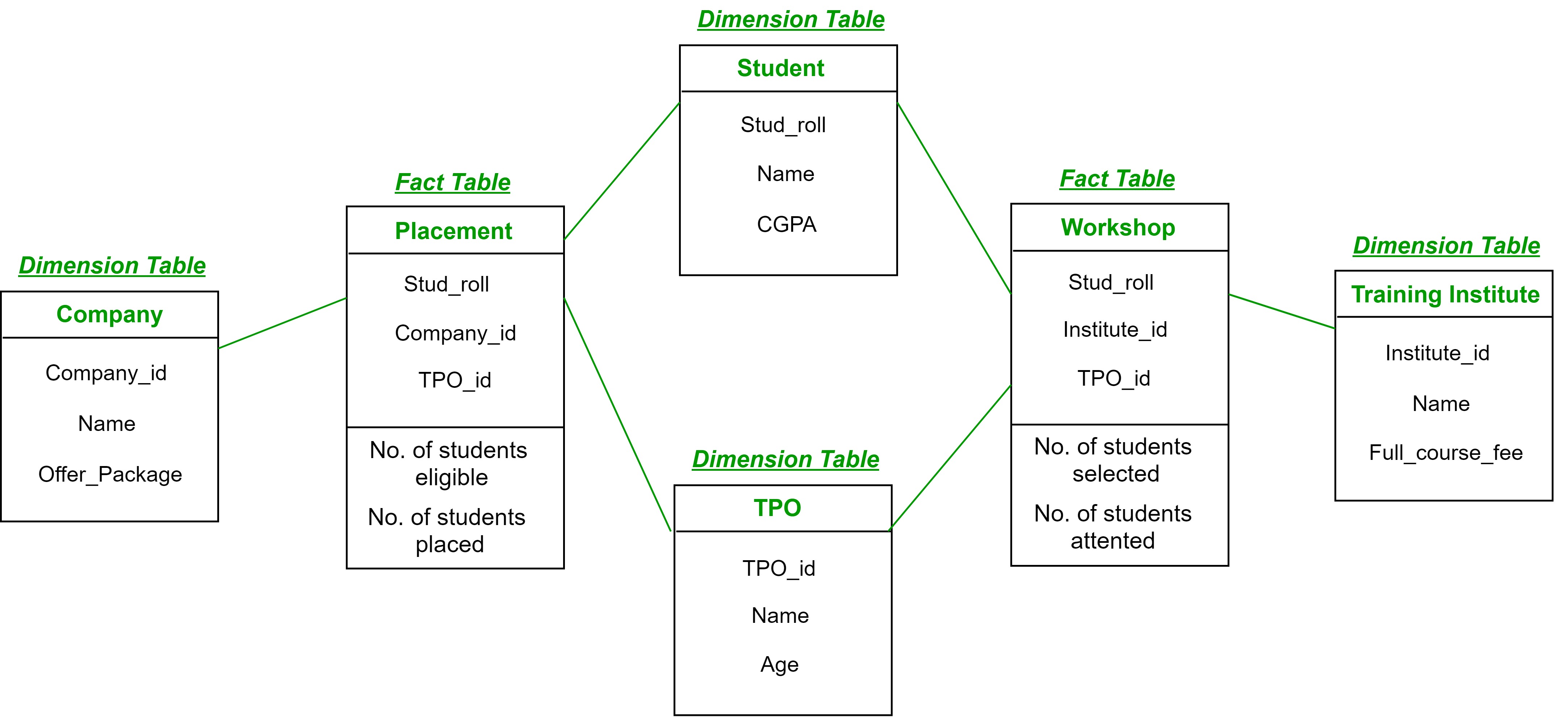
It consists of more than one fact table linked to the dimension tables having attributes. It is also called a fact constellation schema. Conformed dimensions are the dimension tables shared with the fact tables. We can normalize the dimensions in this schema further, but it will lead to a more complex design.

The following diagram shows Placement and Workshop as the two fact tables present. And the dimension table, Student, and TPO are the conformed dimensions.

ADVANTAGES:

1. Flexible schema.

2. Effective analysis and reporting.

DISADVANTAGES:

1. Has huge dimension tables hence resulting in difficulty in managing.

2. Hard to maintain: It is because of their complex design and as there are many fact tables.

DEFINING A STAR SCHEMA IN DMQL FOR THE DIAGRAM BELOW

define cube Placement [Student, TPO, Company]:No. of students eligible = count(eligible_students), No. of students placed = count(placed_students)
define dimension Student as (Stud_roll, Name, CGPA)
define dimension TPO as (TPO_id, Name, Age)
define dimension Company as (Company_id, Name, Offer_Package)

define cube Workshop [Student, TPO, Training Institute]:No. of students selected = count(selected_students), No. of students attended = count(attended_students)
define dimension Student as Student in cube Placement
define dimension TPO as TPO in cube Placement
define dimension Training Institute as (Institute_id, Name, Full_course_fee)

Image Source

Conclusion

In this article, we learned about what schemas are, their different types, and their role in data warehouse modeling. There were some key concepts such as what is a primary key, foreign key, and fact tables. They play an important role in developing an understanding of schemas. Schemas help to see how business concepts relate by designing data models. Hence, they play a huge role in turning raw data into information.

Some of the key takeaways are as follows:

1. Schemas help define relationships between different database tables. A primary key-foreign key relationship forms the link.

2. Normalization and the number of fact tables define what type of schema to form.

3. We view the data in the form of a data cube.

End Notes

Thanks for reading!

Hoping you gained some more knowledge about the topic and enjoyed reading the article.

Feel free to share your thoughts in the comments below or contact me on Linkedin, Email.

The media shown in this article is not owned by Analytics Vidhya and is used at the Author’s discretion.