This article was published as a part of the Data Science Blogathon.

Introduction to Imbalanced Datasets
The accuracy achieved by many of the machine learning models using traditional statistical algorithms increases by just around 2% or so when the size of the training dataset is increased from 20% to 80%. But what about the classification algorithms that mostly deal with imbalanced datasets that already have a very small percentage of minority class? What should be the sample size? or How big should the size of the training dataset be? This article analyses the impact of the size of the training dataset on the various accuracy scores of imbalanced datasets.
The objective is to understand the effectiveness and accuracies of the machine learning algorithms with reference to information sufficiency in terms of the required size of the training dataset, by iterating the models over various scenarios, rather than to arrive at the best possible accuracy for a given dataset.
Imbalanced Datasets
The Imbalanced datasets involve datasets that have a significant deviation of the percentage of rows between the majority and minority classes present. This deviation should be distinguished from the perspective of the machine learning algorithm vs the nature of the real-world problem that is being modelled (1). If the proportion of majority and minority classes does not represent the real-world problem, then our efforts should first be to acquire more data on minority classes.
If additional data on minority classes are not available or if the accuracy of the model is very low implying a lack of sufficient information on minority classes, we may then resort to the synthetic creation of samples of the minority class using methods like SMOTE.
Assuming that we have got a dataset that represents the nature of the real-world problem, we can analyze the effectiveness of the machine learning algorithm with respect to varying sample sizes. The analysis of imbalanced datasets with respect to accuracies achieved vs sample size gives interesting insights that can help us understand the nature of the problem of imbalanced datasets, and allow us to have some insights on choosing the required size of the dataset and also the suitable accuracy measure.
Illustrative Datasets
We shall use Kaggle’s European Credit Card Fraud Detection dataset(2). This dataset consists of 284,807 rows of credit card transactions out of which 492 rows of fraudulent transactions belong to the minority class, constituting just 0.1727% of all transactions. We shall assume that this is the normal percentage of fraudulent transactions that happen in typical credit card transactions in the real world.
In order to verify the results, we also do the same analysis on the protein-homo dataset(3) (can be downloaded from imblearn datasets from scikit imblearn library). This dataset has 145,751 rows with minority classes constituting 1296 (0.889%) rows. The target classifies whether a protein is homologous to a target protein. The graphs pertaining to this dataset are given in the appendix.
Accuracy Measures
Before we start our analysis, we have to decide on the accuracy measure to be used for evaluating the model. The important standard accuracy measures are listed below:
1. Default accuracy – A measure that gives a percentage of total correct predictions, i.e. both genuine and fraudulent transactions, out of all transactions. This gives equal importance to the prediction of both the majority class and minority classes. If the dataset contains 2% fraudulent transactions and the model predicts only 98% of good transactions, then we will get 98% accuracy. Hence, we cannot use this measure.
2. Recall – This is a measure of the percentage of fraudulent transactions (positive class) predicted against all fraudulent transactions in the dataset. This is a measure we should consider in evaluating the model. This is the most important measure since we want all of the fraudulent transactions to be identified correctly. Ideally, we want this score to be 100%
3. Balanced Accuracy – This is the average recall obtained in both classes. Since this considers recall of both good and fraudulent transactions, this is a better measure than the recall if we are interested in the accuracy of both predictions. The credit card company might block transactions that are predicted as fraudulent by the machine learning model. But if a genuine transaction is flagged as fraudulent, then blocking such a transaction could affect customer relationships. Hence, the model should give a good recall for both classes.
If this measure is lower than recall, then it indicates that though the model is predicting well the fraudulent transactions correctly, it is also predicting good transactions as fraudulent, which may not be acceptable.
4. Precision – This is a measure of the percentage of fraudulent transactions predicted against all transactions predicted as fraudulent. This measure will be low when there are many false positives. If this score is low, then it means that the model, even though correctly predicts the fraudulent transactions, is also identifying many genuine transactions as fraudulent.
This score is important in cases where false positives are not accepted in comparison to true positives. For example, in the case of detection of spam emails, we are not bothered much if a spam email is flagged as a good email in comparison to flagging a good email as spam email which we don’t want to happen.
In this article, we will find that the sample size and degree of imbalance have a huge impact on accuracy measures like precision and recall.
5. F1 Score – This is the harmonic mean of the precision and recalls accuracy measures. It gives more weightage to the lower value as compared to the arithmetic mean. If the recall is very high but precision is low, then the f1 score will be lower than the arithmetic average. This measure, in general, will be between the precision and recall scores. If the precision is low, then balanced accuracy will still be high while the f1 score will be low.
If the credit card company wants to give equal importance to both recall (detecting fraudulent transactions) and precision (less false positives), then it should use the f1 score against the balance accuracy score.
Alternatively, if the credit card company wants to give more importance to precision than recall, then it can use the f-beta accuracy measure where we can give higher weightage to the accuracy measure we want to focus on.
6. Area ROC – The area under the Receiver Operating Characteristic curve gives an indication of the effectiveness of the model chosen. A score of 1 indicates a perfect model that makes 100% correct predictions.
Model Scenarios
In this article, an analysis is done with varying sample sizes leading to different models obtained through iteration with the consequent resultant accuracies obtained. The various scenarios considered are:
Scenario 1: Increasing the size of the dataset while keeping the minority classes at the maximum
Using this scenario, we evaluate, given the maximum possible minority class rows, how the size of the majority class impacts the different accuracy scores.
Scenario 2: Increasing the size of the dataset gradually and doing random under-sampling for each iteration of the dataset
Using this scenario, we evaluate the behaviour of accuracies with increasing random under-sampling and whether an optimal size of minority class exists.
Scenario 3: Increasing the size of the dataset gradually with a proportionate number of rows of minority class
Using this scenario, we can analyze the optimal size of the overall training dataset and the behaviour of the accuracies with each iteration
Scenario 4: Increasing the size of the dataset while also increasing the size of the minority classes
Using this scenario, we evaluate the possible optimal size of the minority class required. This is similar to scenario 3 but allows manually choosing the proportion of minority class
The above analyses result in some significant insights that can help us better decide the sample size and the accuracy score to focus on.
Model Algorithm
We use the Random Forest Classifier for evaluation. We may get better accuracies with other algorithms like XGBoost but here our objective is not the magnitude of the accuracy but the behaviour of the accuracies with respect to sample size (although there could be differences in performance between different accuracy measures under different algorithms but here we are more interested in the behaviour of the accuracies with respect to change in sample size which is unlikely to change much between the type of algorithms). We shall also go with the default parameters. No analysis and experimentation with regard to the need for imbalance techniques like SMOTE, Tomek, etc., are implemented as our objective is not to arrive at the maximum possible accuracy for the credit card dataset.
Basic Model
Let us first consider the entire dataset and fit a model with a Random Forest classifier to get the default accuracy measures. The basic model that fits a model with an 80% training dataset, gives a balanced accuracy of 86.22%. The precision and recall are 95.95% and 72.45% respectively.
import pandas as pd
import numpy as np
import matplotlib.pyplot as plt
import seaborn as sns
from sklearn.ensemble import RandomForestClassifier
from sklearn.preprocessing import LabelEncoder
from sklearn.model_selection import cross_val_score
from sklearn.model_selection import RepeatedStratifiedKFold
from sklearn.model_selection import train_test_split
from sklearn.model_selection import cross_validate
from sklearn.metrics import confusion_matrix, accuracy_score
from sklearn.metrics import balanced_accuracy_score
from sklearn.metrics import precision_recall_fscore_support
from sklearn.metrics import f1_score
from sklearn.metrics import classification_report
from sklearn.metrics import roc_curve
from sklearn.metrics import roc_auc_score
from sklearn.metrics import precision_score
from sklearn.metrics import recall_score
from sklearn.metrics import fbeta_score
from imblearn.under_sampling import RandomUnderSampler
from collections import Counter
from imblearn.datasets import make_imbalance
A repeated stratified k-fold cross validation gives the following accuracy scores:
df=pd.read_csv('creditcard.csv')
clf2=RandomForestClassifier()
X2x=df.iloc[:,:-1]
y2x=df.iloc[:,-1]
le2 = LabelEncoder()
y2x = le2.fit_transform(y2x)
X2i_train, X2i_test, y2i_train, y2i_test = train_test_split(X2x, y2x, test_size = 0.2, random_state = 0,stratify=y2x)
splits=5
folds = RepeatedStratifiedKFold(n_splits = splits, n_repeats=3,  random_state = 100)#shuffle = True,
scoresba = cross_val_score(clf2,X2i_train, y2i_train,  n_jobs=-1, cv=folds, scoring='balanced_accuracy')
scoresps = cross_val_score(clf2,X2i_train, y2i_train,  n_jobs=-1, cv=folds, scoring='precision')
scoresrc = cross_val_score(clf2,X2i_train, y2i_train,  n_jobs=-1, cv=folds, scoring='recall')
scoresf1 = cross_val_score(clf2,X2i_train, y2i_train,  n_jobs=-1, cv=folds, scoring='f1')
print("The BA score of Repeated stratified Kfold with ",splits,"splits is n",scoresba.min(),scoresba.mean(),scoresba.max())
print("The PS score of Repeated stratified Kfold with ",splits,"splits is n",scoresps.min(),scoresps.mean(),scoresps.max())
print("The RC score of Repeated stratified Kfold with ",splits,"splits is n",scoresrc.min(),scoresrc.mean(),scoresrc.max())
print("The F1 score of Repeated stratified Kfold with ",splits,"splits is n",scoresf1.min(),scoresf1.mean(),scoresf1.max())
The BA score of Repeated stratified Kfold with  5 splits is
 0.8653186682741979 0.8958838670842708 0.9366868779061193
The PS score of Repeated stratified Kfold with  5 splits is
 0.9047619047619048 0.9485453383389694 0.9855072463768116
The RC score of Repeated stratified Kfold with  5 splits is
 0.7307692307692307 0.7909985935302392 0.8607594936708861
The F1 score of Repeated stratified Kfold with  5 splits is
 0.8142857142857143 0.8635234484817464 0.9261744966442954
The basic model gives a default balanced accuracy score of 89.59%.
Now, let us analyze the changes in the above accuracies with different sample sizes.
Analysis of Scenarios and Key Insights
By creating several models based on the various scenarios listed earlier, we arrive at several insights. These insights are explained below:
Scenario 1 – Increasing the size of the dataset while keeping the minority classes at the maximum
Results: Insight A – The accuracy of the machine learning algorithms decreases with the increase in sample size for imbalanced datasets
The effectiveness of the machine learning algorithm depends on the degree of imbalance in the dataset. This means that given the size of the minority class if the rows in majority classes are increased, the balanced accuracy decreases. This is shown in the following illustration.
The code below creates a model that iteratively increases the size of the training dataset while keeping the size of the minority class at the maximum.
The graph below shows that as the sample size increases for the given fixed number of rows of the minority class, the balanced accuracy and other measures decrease gradually.
df=pd.read_csv('creditcard.csv')
clf2=RandomForestClassifier()
X2=df.iloc[:,:-1]
y2=df.iloc[:,-1]
# Split the dataset into training and test data set
X2i_train, X2i_test, y2i_train, y2i_test = train_test_split(X2, y2, test_size = 0.2, random_state = 0,stratify=y2)
# For the extracted training dataset, find out the maximum size of minority class.
# This shall be kept constant in each iteration
xz=pd.DataFrame(y2i_train)
j=xz.loc[xz['Class']==1].shape[0]
e=X2i_train.shape[0]-j
# Initialize lists for storing the accuracy scores so that graphs can be plotted
bac=[];ac=[];xl=[];fa=[];aroc=[];pss=[];rss=[];fbs=[];fb5s=[]
# Extract different training dataset from the initial training dataset by iterating by increments of 1000
for i in range(j,e,5000):
    X2=df.iloc[:,:-1]
    y2=df.iloc[:,-1]
    le2 = LabelEncoder()
    y2 = le2.fit_transform(y2)
    X2i_train, X2i_test, y2i_train, y2i_test = train_test_split(X2, y2, test_size = 0.2, random_state = 0,stratify=y2)
    # Create a sample dataset with fixed j number of minority rows and increasing majority class in each iteration
    X2, y2 = make_imbalance(X2i_train,y2i_train,sampling_strategy={0:i,1:j})
    #Build a model using the extracted dataset
    clf2.fit(X2,y2)
    pred_y2=clf2.predict(X2i_test)
    # calculate and store accuracy scores
    bacc=balanced_accuracy_score(y2i_test,pred_y2)
    acc=accuracy_score(y2i_test,pred_y2)
    ps=precision_score(y2i_test,pred_y2)
    rs=recall_score(y2i_test,pred_y2)
    fb2=fbeta_score(y2i_test,pred_y2,beta=2)
    fb05=fbeta_score(y2i_test,pred_y2,beta=0.5)
    f1=f1_score(y2i_test, pred_y2)
    probs=clf2.predict_proba(X2i_test)
    r=roc_auc_score(y2i_test,probs[:,1])
    xl.append(len(X2))
    bac.append(bacc)
    ac.append(acc)
    fa.append(f1)
    pss.append(ps)
    rss.append(rs)
    fbs.append(fb2)
    fb5s.append(fb05)
    aroc.append(r)
    #Print the scores
    cm = confusion_matrix(y2i_test, pred_y2)
    print("Confusion Matrix for Test Data n",cm)
    print("Accuracy Score for Test Data n", acc)#accuracy_score(y2i_test,pred_y2))
    print("Balanced accuracy Score for Test Data n", bacc)#balanced_accuracy_score(y2i_test,pred_y2))
    print("F1 Accuracy Score for Test Data n", f1)#f1_score(y2i_test,pred_y2,average='macro'))
    print("Area under ROC Score n",r)
    print("Precision Accuracy Score for Test Data n",ps )
    print("Recall Accuracy Score for Test Data n", rs)
    print("F-Beta Accuracy Score for Test Data n", fb2)
    print("F-Beta Accuracy Score for Test Data n", fb05)
    print("F1 Accuracy Score for Test Data n", f1)
    print("The Area under ROC Curve is ",r)
    print("Length of X here in loop is n",i)
# Plot the graphs
yz=pd.DataFrame(y2)
print("Y2 Value counts is n",yz.value_counts())
print("Accuracy Score   ",acc)
print("balanced Accuracy Score   ",bacc)
print("Length of X ",i)
print("Maximum Balanced Accuracy is ",max(bac))
print("Maximum Precision Score is ",max(pss))
print("Maximum Recall score is ",max(rss))
print("Maximum F Beta score is ",max(fbs))
print("Maximum F Beta score is ",max(fb5s))
print("Maximum Area under Curve is ",max(aroc))
sns.regplot(x=xl, y=ac,lowess=True,  label='Accuracy')
sns.regplot(x=xl, y=bac, lowess=True, label='Balanced Accuracy')
sns.regplot(x=xl, y=fa, lowess=True, label='F1 Score')
sns.regplot(x=xl, y=aroc, lowess=True, label='Area under ROC curve')
sns.regplot(x=xl, y=pss, lowess=True, label='Precision Score')
sns.regplot(x=xl, y=rss, lowess=True, label='Recall Score')
sns.regplot(x=xl, y=fbs, lowess=True, label='F-Beta Score-2')
sns.regplot(x=xl, y=fb5s, lowess=True, label='F-Beta Score-0.5')
plt.title('Accuracy', fontsize=16)
plt.xlabel('Sample Size')
plt.ylabel('Accuracy')
plt.legend()
plt.savefig("Credit-card-ConstY2306.png")
plt.show()
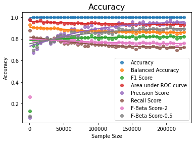

Maximum Balanced Accuracy is  0.9286724573059386
Maximum Precision Score is  0.9726027397260274
Maximum Recall score is  0.8775510204081632
Maximum F Beta score is  0.802469135802469
Maximum F Beta score is  0.9102564102564104
Maximum Area under Curve is  0.976034835712563
The second graph above clearly shows that the balanced accuracy decreases as the degree of imbalance increases – in this case, we kept the rows of minority class to a maximum, and kept increasing the rows of the majority class. We can also statistically validate this inverse linear relationship with python functions:
import minepy
from minepy import MINE
mine = MINE(alpha=0.6, c=15, est="mic_approx")
mine.compute_score(xl, bac)
print("Pearson correlation coefficient between sample size and
balanced accuracy is ","{:.2f}".format(np.corrcoef(xl,bac)[0,1]))
print("Maximal Information Criterion
between sample size and balanced accuracy is ","{:.2f}".format(mine.mic()))
Pearson correlation coefficient between sample size and balanced accuracy is  -0.87
Maximal Information Criterion between sample size and balanced accuracy is  1.00
Thus, as the degree of imbalance increases the accuracy measure decreases.
Another important insight we can get from the output of the above model and the graphs is that the precision increases significantly as the sample size increases at the cost of the recall. This can be seen by looking at the those two graphs
Results – Insight B: With a constant size of the minority class, if the sample size is increased, the precision increases while recall decreases
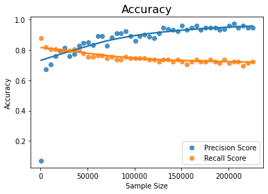
Precision increases with sample size for constant minority class while recall decreases
The statistical measure of the linear dependence also shows that the precision indeed increases with the sample size
mine.compute_score(xl, pss)
print("Pearson correlation coefficient between sample size and
precision score is ","{:.2f}".format(np.corrcoef(xl,pss)[0,1]))
print("Maximal Information Criterion
between sample size and precision score is ","{:.2f}".format(mine.mic()))
Pearson correlation coefficient between sample size and precision score is  0.64
Maximal Information Criterion between sample size and precision score is  1.00
Insight A above means that we should have the rows of majority classes as less as possible if our objective is mainly the accuracy measure of balanced_accuracy and recall.
How many majority classes should we have? Maximum accuracy can be obtained when imbalance is zero which means the number of rows of majority and minority classes are the same. This implies the maximum accuracy can be obtained with random under-sampling method of sci-kit learn library
Random Undersampling
The code below gives the accuracy with random under-sampling:
df=pd.read_csv('creditcard.csv')
clf2=RandomForestClassifier()
X2x=df.iloc[:,:-1]
y2x=df.iloc[:,-1]
le2 = LabelEncoder()
y2x = le2.fit_transform(y2x)
X2i_train, X2i_test, y2i_train, y2i_test = train_test_split(X2x, y2x, test_size = 0.2, random_state = 0,stratify=y2x)
rus = RandomUnderSampler(random_state=534534, replacement=True)
X2,y2 = rus.fit_resample(X2i_train,y2i_train)
print('original dataset shape:', Counter(y2i_train))
print('Resample dataset shape', Counter(y2))
y2df=pd.Series(y2)
y2l=y2df.shape[0]
print("y2 length here n",y2l)
clf2.fit(X2,y2)
pred_y2=clf2.predict(X2i_test)
bacc=balanced_accuracy_score(y2i_test,pred_y2)
acc=accuracy_score(y2i_test,pred_y2)
ps=precision_score(y2i_test,pred_y2)
rs=recall_score(y2i_test,pred_y2)
fb2=fbeta_score(y2i_test,pred_y2,beta=2)
fb05=fbeta_score(y2i_test,pred_y2,beta=0.5)
f1=f1_score(y2i_test, pred_y2)
probs=clf2.predict_proba(X2i_test)
f,t,th=roc_curve(y2i_test,probs[:,1],pos_label=1,drop_intermediate=False)
r=roc_auc_score(y2i_test,probs[:,1])
cm = confusion_matrix(y2i_test, pred_y2)
print("Confusion Matrix for Test Data n",cm)
print("Accuracy Score for Test Data n", acc)#accuracy_score(y2i_test,pred_y2))
print("Balanced accuracy Score for Test Data n", bacc)#balanced_accuracy_score(y2i_test,pred_y2))
print("F1 Accuracy Score for Test Data n", f1)#f1_score(y2i_test,pred_y2,average='macro'))
print("Precision Accuracy Score for Test Data n",ps )
print("Recall Accuracy Score for Test Data n", rs)
print("F-Beta Accuracy Score for Test Data n", fb2)
print("F-Beta Accuracy Score for Test Data n", fb05)
print("F1 Accuracy Score for Test Data n", f1)
print(classification_report(y2i_test, pred_y2))
The output of the above code is given below:
original dataset shape: Counter({0: 227451, 1: 394})
Resample dataset shape Counter({0: 394, 1: 394})
y2 length here
 788
Confusion Matrix for Test Data
 [[55605  1259]
 [   13    85]]
Accuracy Score for Test Data
 0.9776693234085881
Balanced accuracy Score for Test Data
 0.9226031964558474
F1 Accuracy Score for Test Data
 0.11789181692094312
Precision Accuracy Score for Test Data
 0.06324404761904762
Recall Accuracy Score for Test Data
 0.8673469387755102
F-Beta Accuracy Score for Test Data
 0.24481566820276499
F-Beta Accuracy Score for Test Data
 0.07763975155279504
F1 Accuracy Score for Test Data
 0.11789181692094312
              precision    recall  f1-score   support
           0       1.00      0.98      0.99     56864
           1       0.06      0.87      0.12        98
    accuracy                           0.98     56962
   macro avg       0.53      0.92      0.55     56962
weighted avg       1.00      0.98      0.99     56962
Note that the simple random under-sampling with just 788 rows of data gives a balanced accuracy of 92.26% which is far higher than the balanced accuracy of 89.58% obtained with entire 2 lac rows of data.
Now, we may ask if the recall accuracy is greatest when the degree of imbalance is zero that can be achieved by random under-sampling, what should be the optimal size of the minority class?
To analyze this, we create another scenario of the iterative model.
Scenario 2 – Random Under Sampling with gradual increase of sample size
We build a new iterative modelling scenario where we iterate over the training dataset by gradually increasing the training dataset size. For each training dataset size, we do random under-sampling. The code is given below for this scenario:
df=pd.read_csv('creditcard.csv')
clf2=RandomForestClassifier()
# Initialize lists for storing the accuracy scores so that graphs can be plotted
bac=[];ac=[];xl=[];fa=[];aroc=[];pss=[];rss=[];fbs=[];fb5s=[]
for i in range(1,40,1):
    print(i)
    X2x=df.iloc[:,:-1]
    y2x=df.iloc[:,-1]
    le2 = LabelEncoder()
    y2x = le2.fit_transform(y2x)
    X2i_train, X2i_test, y2i_train, y2i_test = train_test_split(X2x, y2x, test_size = 0.2, random_state = 0,stratify=y2x)
    X2_train, X2_test, y2_train, y2_test = train_test_split(X2i_train, y2i_train, train_size = i/40,shuffle=y2i_train)
    rus = RandomUnderSampler(random_state=234354, replacement=True)
    X2,y2 = rus.fit_resample(X2_train,y2_train)
    print('original dataset shape:', Counter(y2_train))
    print('Resample dataset shape', Counter(y2))
    y2df=pd.Series(y2)
    y2l=y2df.shape[0]
    print("y2 length here n",y2l)
    clf2.fit(X2,y2)
    pred_y2=clf2.predict(X2i_test)
    bacc=balanced_accuracy_score(y2i_test,pred_y2)
    acc=accuracy_score(y2i_test,pred_y2)
    probs=clf2.predict_proba(X2i_test)
    r=roc_auc_score(y2i_test,probs[:,1])
    ps=precision_score(y2i_test,pred_y2)
    rs=recall_score(y2i_test,pred_y2)
    fb2=fbeta_score(y2i_test,pred_y2,beta=2)
    fb05=fbeta_score(y2i_test,pred_y2,beta=0.5)
    f1=f1_score(y2i_test, pred_y2)
    xl.append(y2l)
    bac.append(bacc)
    ac.append(acc)
    fa.append(f1)
    pss.append(ps)
    rss.append(rs)
    fbs.append(fb2)
    fb5s.append(fb05)
    aroc.append(r)
    cm = confusion_matrix(y2i_test, pred_y2)
    print("Confusion Matrix for Test Data n",cm)
    print("Accuracy Score for Test Data n", acc)#accuracy_score(y2i_test,pred_y2))
    print("Balanced accuracy Score for Test Data n", bacc)#balanced_accuracy_score(y2i_test,pred_y2))
    print("F1 Accuracy Score for Test Data n", f1)#f1_score(y2i_test,pred_y2,average='macro'))
    print("Precision Accuracy Score for Test Data n",ps )
    print("Recall Accuracy Score for Test Data n", rs)
    print("F-Beta Accuracy Score for Test Data n", fb2)
    print("F-Beta Accuracy Score for Test Data n", fb05)
    print("F1 Accuracy Score for Test Data n", f1)
yz=pd.DataFrame(y2)
print("Y2 Value counts is n",yz.value_counts())
print("Accuracy Score   ",acc)
print("balanced Accuracy Score   ",bacc)
print("Length of X ",i)
print("Maximum Balanced Accuracy is ",max(bac))
print("Maximum Precision Score is ",max(pss))
print("Maximum Recall score is ",max(rss))
print("Maximum F Beta score is ",max(fbs))
print("Maximum F Beta score is ",max(fb5s))
print("Maximum Area under Curve is ",max(aroc))
sns.regplot(x=xl, y=ac,lowess=True,  label='Accuracy')
sns.regplot(x=xl, y=bac, lowess=True, label='Balanced Accuracy')
sns.regplot(x=xl, y=fa, lowess=True, label='F1 Score')
sns.regplot(x=xl, y=aroc, lowess=True, label='Area under ROC curve')
sns.regplot(x=xl, y=pss, lowess=True, label='Precision Score')
sns.regplot(x=xl, y=rss, lowess=True, label='Recall Score')
sns.regplot(x=xl, y=fbs, lowess=True, label='F-Beta Score-2')
sns.regplot(x=xl, y=fb5s, lowess=True, label='F-Beta Score-0.5')
plt.title('Accuracy', fontsize=16)
plt.xlabel('Sample Size')
plt.ylabel('Accuracy')
plt.legend()
plt.savefig("CC-Model-RUS.png")
plt.show()
The maximum accuracy measures of the output of the above code are given below
Maximum Balanced Accuracy is  0.9289010729502831
Maximum Precision Score is  0.425414364640884
Maximum Recall score is  0.8877551020408163
Maximum F Beta score is  0.6719022687609075
Maximum F Beta score is  0.46836982968369834
Maximum Area under Curve is  0.9818369895088029
The various accuracy graphs are shown below:

The above graph shows that the increase in the size of the random under-sample (i.e. size of the minority class) does not improve the accuracy much as the graph is nearly flat. This is seen more clearly in the following graph that plots balanced accuracy and recall alone

The correlation between sample size and the recall / balanced accuracy measures also shows the relationship is weak for increasing the size of random under-sampling:
from minepy import MINE
mine = MINE(alpha=0.6, c=15, est="mic_approx")
mine.compute_score(xl, bac)
print("Pearson correlation coefficient between sample size and
balanced_accuracy score is ","{:.2f}".format(np.corrcoef(xl,bac)[0,1]))
print("Maximal Information Criterion
between sample size and balanced_accuracy score is ","{:.2f}".format(mine.mic()))
mine.compute_score(xl, rss)
print("Pearson correlation coefficient between sample size and
recall score is ","{:.2f}".format(np.corrcoef(xl,rss)[0,1]))
print("Maximal Information Criterion
between sample size and recall score is ","{:.2f}".format(mine.mic()))
Pearson correlation coefficient between sample size and balanced_accuracy score is  0.36
Maximal Information Criterion between sample size and balanced_accuracy score is  0.35
Pearson correlation coefficient between sample size and recall score is  0.35
Maximal Information Criterion between sample size and recall score is  0.39
The above insights mean that we can get higher accuracies with even a small sample size of minority class!!
How much smaller should that be?
A partial output of the above code is given below (for training dataset size of 52 rows and minority class size of 26 rows):
original dataset shape: Counter({0: 17062, 1: 26})
Resample dataset shape Counter({0: 26, 1: 26})
y2 length here
 52
Confusion Matrix for Test Data
 [[55512  1352]
 [   14    84]]
Accuracy Score for Test Data
 0.9760191004529335
Balanced accuracy Score for Test Data
 0.9166834150655196
F1 Accuracy Score for Test Data
 0.10951760104302476
Precision Accuracy Score for Test Data
 0.0584958217270195
Recall Accuracy Score for Test Data
 0.8571428571428571
F-Beta Accuracy Score for Test Data
 0.2297592997811816
F-Beta Accuracy Score for Test Data
 0.07189318726463538
F1 Accuracy Score for Test Data
 0.10951760104302476
It can be seen from the output excerpt from the above model that a random under-sampling of a training dataset of size 52 rows gives an accuracy that is comparable to the accuracy of 200,000 rows of data!
If we can get such a high accuracy with the small size of the dataset with random under-sampling, what is it that we lose? The downfall of random under-sampling is the precision accuracy score. The precision accuracy score becomes very low even while the recall score is high. This can be seen from the graph below – while the recall scores are above 80%, the precision scores are below 20%.
Alternatively, we can say that when the rows of the majority classes are reduced to decrease the degree of imbalance, the precision becomes very low
When we do random under-sampling, the recall accuracy goes very high but the precision takes a beating. The low precision score means that some of the genuine transactions are categorized as fraudulent. This is highly undesirable as good customers will be affected, and the transaction might get blocked.
Hence, if the bank does not want genuine transactions to be classified as fraudulent, then the random under-sampling method should not be used.
Result – Insight C – We should not go for random under-sampling if we are interested in the precision score as against the recall score
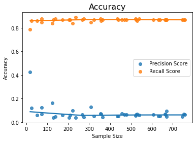
This insight means that we can reduce training dataset size to reduce the degree of imbalance for doing random under-sampling ONLY if our objective is to improve the recall score and we are not bothered about the precision score.
Scenario 3 – The increasing size of training dataset size with the same proportion or degree of imbalance
In this scenario, we iterate over several models with increasing size of the training dataset within the extracted training dataset, while keeping the 20% of the dataset for testing so that there is no data leakage.
Results – Insight D – As the sample size (or size of training dataset) is increased with the same proportion of the minority class, the precision increases but recall goes down
This is illustrated in the following example. The maximum scores and accuracy graphs are given below.
df=pd.read_csv('creditcard.csv')
clf2=RandomForestClassifier()
# Initialize lists for storing the accuracy scores so that graphs can be plotted
bac=[];ac=[];xl=[];fa=[];aroc=[];pss=[];rss=[];fbs=[];fb5s=[]
# Extract 20 training sets of increasing size and predict test data using each model
for i in range(1,40,1):
    print(i)
    X2x=df.iloc[:,:-1]
    y2x=df.iloc[:,-1]
    le2 = LabelEncoder()
    y2x = le2.fit_transform(y2x)
    X2i_train, X2i_test, y2i_train, y2i_test = train_test_split(X2x, y2x, test_size = 0.2, random_state = 0,stratify=y2x)
    X2_train, X2_test, y2_train, y2_test = train_test_split(X2i_train, y2i_train, train_size = i/40,shuffle=y2i_train)
    clf2.fit(X2_train,y2_train)
    pred_y2=clf2.predict(X2i_test)
    bacc=balanced_accuracy_score(y2i_test,pred_y2)
    acc=accuracy_score(y2i_test,pred_y2)
    ps=precision_score(y2i_test,pred_y2)
    rs=recall_score(y2i_test,pred_y2)
    fb2=fbeta_score(y2i_test,pred_y2,beta=2)
    fb05=fbeta_score(y2i_test,pred_y2,beta=0.5)
    f1=f1_score(y2i_test, pred_y2)
    probs=clf2.predict_proba(X2i_test)
    r=roc_auc_score(y2i_test,probs[:,1])
    xl.append(len(X2_train))
    bac.append(bacc)
    ac.append(acc)
    fa.append(f1)
    pss.append(ps)
    rss.append(rs)
    fbs.append(fb2)
    fb5s.append(fb05)
    aroc.append(r)
    cm = confusion_matrix(y2i_test, pred_y2)
    print("Confusion Matrix for Test Data n",cm)
    print("Accuracy Score for Test Data n", acc)#accuracy_score(y2i_test,pred_y2))
    print("Balanced accuracy Score for Test Data n", bacc)#balanced_accuracy_score(y2i_test,pred_y2))
    print("F1 Accuracy Score for Test Data n", f1)#f1_score(y2i_test,pred_y2,average='macro'))
    print("Precision Accuracy Score for Test Data n",ps )
    print("Recall Accuracy Score for Test Data n", rs)
    print("F-Beta Accuracy Score for Test Data n", fb2)
    print("F-Beta Accuracy Score for Test Data n", fb05)
    print("F1 Accuracy Score for Test Data n", f1)
    print("Length of X here in loop is n",i)
yz=pd.DataFrame(y2_train)
print("Y2 Value counts is n",yz.value_counts())
print("Accuracy Score   ",acc)
print("balanced Accuracy Score   ",bacc)
print("Length of X ",i)
print("Maximum Balanced Accuracy is ",max(bac))
print("Maximum Precision Score is ",max(pss))
print("Maximum Recall score is ",max(rss))
print("Maximum F Beta score is ",max(fbs))
print("Maximum F Beta score is ",max(fb5s))
print("Maximum Area under Curve is ",max(aroc))
sns.regplot(x=xl, y=ac,lowess=True,  label='Accuracy')
sns.regplot(x=xl, y=bac, lowess=True, label='Balanced Accuracy')
sns.regplot(x=xl, y=fa, lowess=True, label='F1 Score')
sns.regplot(x=xl, y=aroc, lowess=True, label='Area under ROC curve')
sns.regplot(x=xl, y=pss, lowess=True, label='Precision Score')
sns.regplot(x=xl, y=rss, lowess=True, label='Recall Score')
sns.regplot(x=xl, y=fbs, lowess=True, label='F-Beta Score-2')
sns.regplot(x=xl, y=fb5s, lowess=True, label='F-Beta Score-0.5')
plt.title('Accuracy', fontsize=16)
plt.xlabel('Sample Size')
plt.ylabel('Accuracy')
plt.legend()
plt.savefig("CC-Model2-IncrTS.png")
plt.show()
The partial output of the code and graphs of accuracies are given below:
Maximum Balanced Accuracy is  0.8622185192309901
Maximum Precision Score is  0.9722222222222222
Maximum Recall score is  0.7244897959183674
Maximum F Beta score is  0.7618025751072962
Maximum F Beta score is  0.9067357512953367
Maximum Area under Curve is  0.947277715250422
Maximum Area under Curve is  0.947277715250422
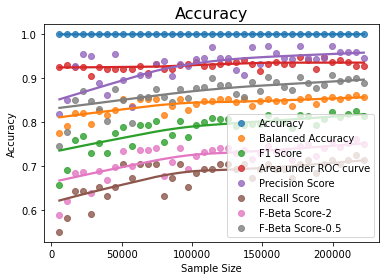
The graphs above show that if we increase the size of the training dataset with the same proportion of minority and majority classes since the degree of imbalance is maintained, the recall score is low as noted already, but the precision score becomes very high.
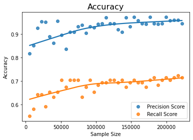
If the training dataset is increased, the precision score increases
mine.compute_score(xl, pss)
print("Pearson correlation coefficient between sample size and
precision accuracy score is ","{:.2f}".format(np.corrcoef(xl,pss)[0,1]))
print("Maximal Information Criterion
between sample size and balanced_accuracy score is ","{:.2f}".format(mine.mic()))
mine.compute_score(xl, rss)
print("Pearson correlation coefficient between sample size and
recall score is ","{:.2f}".format(np.corrcoef(xl,rss)[0,1]))
print("Maximal Information Criterion
between sample size and recall score is ","{:.2f}".format(mine.mic()))
Pearson correlation coefficient between sample size and precision accuracy score is  0.62
Maximal Information Criterion between sample size and balanced_accuracy score is  0.52
Pearson correlation coefficient between sample size and recall score is  0.72
Maximal Information Criterion between sample size and recall score is  0.55
The above insight implies that if the objective is to increase precision over recall, then the size of the training set should be maximum in order to increase precision.
For example, consider spam email detection. In this case, while we want to ensure that a spam email is correctly detected, we don’t want a good email to be classified as spam. This means we want the highest precision possible. Hence, in such cases, we need to have as much data on the majority class as possible.
If our interest is precision score as against recall, as in the case of spam detection, we may be interested in knowing the size of the training dataset and the minority class that is required at which the precision score reaches maximum. It is not necessary that it has to be at the maximum dataset size. This can be analyzed to some extent using the next scenario
Scenario 4 – Increasing minority sample size along with training dataset size
We can analyze the behaviour of precision score, by increasing the training dataset size along with the size of the minority class.
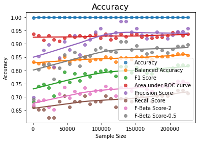
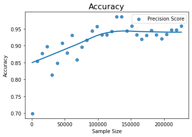
Result – Insight E – As the size of the training dataset size along with size of minority class is increased, the precision increases
df=pd.read_csv('creditcard.csv')
clf2=RandomForestClassifier()
X2=df.iloc[:,:-1]
y2=df.iloc[:,-1]
le2 = LabelEncoder()
y2 = le2.fit_transform(y2)
X2i_train, X2i_test, y2i_train, y2i_test = train_test_split(X2, y2, test_size = 0.2, random_state = 0,stratify=y2)
j=13
e=X2i_train.shape[0]-j
# Initialize lists for storing the accuracy scores so that graphs can be plotted
bac=[];ac=[];xl=[];fa=[];aroc=[];pss=[];rss=[];fbs=[];fb5s=[]
for i in range(750,227846,7500):
    X2, y2 = make_imbalance(X2i_train,y2i_train,sampling_strategy={0:i,1:j})
    j+=13
    if j>=393:
        j=393
    print(i,j,e)
    clf2.fit(X2,y2)
    pred_y2=clf2.predict(X2i_test)
    bacc=balanced_accuracy_score(y2i_test,pred_y2)
    acc=accuracy_score(y2i_test,pred_y2)
    ps=precision_score(y2i_test,pred_y2)
    rs=recall_score(y2i_test,pred_y2)
    fb2=fbeta_score(y2i_test,pred_y2,beta=2)
    fb05=fbeta_score(y2i_test,pred_y2,beta=0.5)
    probs=clf2.predict_proba(X2i_test)
    r=roc_auc_score(y2i_test,probs[:,1])
    f1=f1_score(y2i_test, pred_y2)
    xl.append(len(X2))
    bac.append(bacc)
    ac.append(acc)
    fa.append(f1)
    pss.append(ps)
    rss.append(rs)
    fbs.append(fb2)
    fb5s.append(fb05)
    aroc.append(r)
    cm = confusion_matrix(y2i_test, pred_y2)
    print("Confusion Matrix for Test Data n",cm)
    print("Accuracy Score for Test Data n", acc)#accuracy_score(y2i_test,pred_y2))
    print("Balanced accuracy Score for Test Data n", bacc)#balanced_accuracy_score(y2i_test,pred_y2))
    print("F1 Accuracy Score for Test Data n", f1)#f1_score(y2i_test,pred_y2,average='macro'))
    print("Area under ROC Score n",r)
    print("Precision Accuracy Score for Test Data n",ps )
    print("Recall Accuracy Score for Test Data n", rs)
    print("F-Beta Accuracy Score for Test Data n", fb2)
    print("F-Beta Accuracy Score for Test Data n", fb05)
    print("F1 Accuracy Score for Test Data n", f1)
    print("The Area under ROC Curve is ",r)
    print("Length of X here in loop is n",i)
yz=pd.DataFrame(y2)
print("Y2 Value counts is n",yz.value_counts())
print("Accuracy Score   ",acc)
print("balanced Accuracy Score   ",bacc)
print("Length of X ",i)
print("Maximum Balanced Accuracy is ",max(bac))
print("Maximum Precision Score is ",max(pss))
print("Maximum Recall score is ",max(rss))
print("Maximum F Beta score is ",max(fbs))
print("Maximum F Beta score is ",max(fb5s))
print("Maximum Area under Curve is ",max(aroc))
sns.regplot(x=xl, y=ac,lowess=True,  label='Accuracy')
sns.regplot(x=xl, y=bac, lowess=True, label='Balanced Accuracy')
sns.regplot(x=xl, y=fa, lowess=True, label='F1 Score')
sns.regplot(x=xl, y=aroc, lowess=True, label='Area under ROC curve')
sns.regplot(x=xl, y=pss, lowess=True, label='Precision Score')
sns.regplot(x=xl, y=rss, lowess=True, label='Recall Score')
sns.regplot(x=xl, y=fbs, lowess=True, label='F-Beta Score-2')
sns.regplot(x=xl, y=fb5s, lowess=True, label='F-Beta Score-0.5')
plt.title('Accuracy', fontsize=16)
plt.xlabel('Sample Size')
plt.ylabel('Accuracy')
plt.legend()
plt.savefig("CC-Model3-IncY.png")
plt.show()
mine.compute_score(xl, pss)
print("Pearson correlation coefficient between sample size and
precision score is ","{:.2f}".format(np.corrcoef(xl,pss)[0,1]))
print("Maximal Information Criterion
between sample size and precision score is ","{:.2f}".format(mine.mic()))
Pearson correlation coefficient between sample size and precision score is  0.67
Maximal Information Criterion between sample size and precision score is  0.79

Since precision is affected by a number of majority rows while recall is dependent on minority class rows as indicated by previous insights, we may try to increase the size of both minority and majority classes so that precision improves as the size of the training dataset increases. The above scenario is presented only as additional support for the previous model and further research/analysis can be done along these lines.
Conclusion to Imbalanced Datasets
In my earlier article(1), I differentiated between the concept of imbalance with respect to machine learning algorithms vs the nature of real-world problems that are represented by the datasets. The nature of machine learning algorithms is such that the accuracy of the predictions decreases with an increase in the degree of imbalance. The degree of imbalance increases with the increase in sample size given the initial size of the minority class. In this article, we further explored the behaviour of the accuracies with different sizes of training sample data and derived some significant insights that would help in modelling imbalanced datasets.
The key insights are:
4. As the sample size (or size of training dataset) is increased with the same proportion of the minority class, the precision increases but recall goes down.
Given a constant size of the minority class, as the size of the majority class increases, the balanced accuracy decreases. This implies that as the degree of imbalance increases, the accuracy decreases. Hence, the random under-sampling technique will always give better accuracy than the overall dataset. If we do random under-sampling with increasing sample size, the balanced accuracy increases. Depending on the information sufficiency, we may reach a size of minority class that may be sufficient to give higher accuracy. If we increase the training set with a proportionate increase in minority class, the precision accuracy becomes very high greater than balanced accuracy while recall is lowest. This insight can be used when the objective of the model is precision over recall like spam detection.
References
1. Is Adult Income Dataset Imbalanced? – https://www.analyticsvidhya.com/blog/2022/06/is-adult-income-dataset-imbalanced/
2. Credit Card Fraud Detection, Kaggle, https://www.kaggle.com/datasets/mlg-ulb/creditcardfraud
3. Particle Physics: plus protein homology, https://www.kdd.org/kdd-cup/view/kdd-cup-2004/Data
The media shown in this article is not owned by Analytics Vidhya and is used at the Author’s discretion.


