Market Basket Analysis for Coffee Shop with Apriori

This article was published as a part of the Data Science Blogathon.

Introduction

A supermarket store named Big Mart opened a coffee shop inside the premises, and after the launch, it started seeing great transactions, and it was decided to have similar coffee shops at all the stores across the region for Big Mart. Big Mart has been using association rules for its main retail stores, and under the marketing plan for these coffee shops, they want to create similar association rules and do combo offers for these shops.

Transaction data for the coffee shop relating to 9000+ purchases were collected. The task is to find out the top association rules for the product team to create combo offers and use the insights to make the coffee shop even more profitable at all these stores.

Reading Dataset

import pandas as pd
import numpy as np
#import warnings
import seaborn as sns
import datetime
import matplotlib.pyplot as plt
#warnings.filterwarnings('ignore')

# Reading the transactions from csv file
df = pd.read_csv('coffeeshop_transactions.csv')

 

Basic Exploration

# Eyeballing a sample of the dataset
df.head(10)

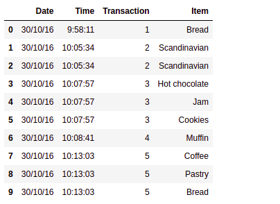
Here, we see the date and time of each transaction with a transaction id in the column called a transaction. We see that transaction 1 just has 1 item of bread, transaction 2 has 2 Scandinavians, and transaction 3 has 3 different items.

Checking for missing values

Checking the number of purchases and missing values

df.shape, #df.info()

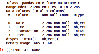
Clearly, there are no missing values here which are great!

Listing all the items in the dataset

#Number of unique Items
df['Item'].nunique()

# Checking the list of items in the dataset
df['Item'].unique()

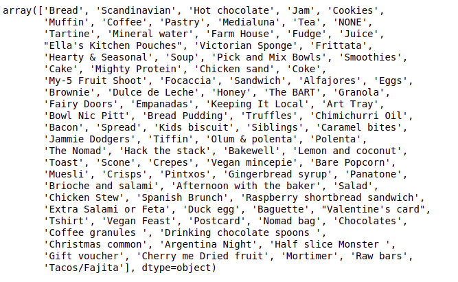
We have a total of 93 items, with one of the items being ‘NONE.’ Let’s check how many rows have ‘NONE’ as the item

#Check how many rows have none as an item
x = df['Item'] == "NONE"
print(x.value_counts())

So there are 786 transactions with none, which is quite small wrt the database, so it would be best to get rid of all these rows.

Dropping all none values from the data frame

#Dropping rows with NONE as the item
df = df.drop(df[df.Item == 'NONE'].index)

Now, given that this is taken care of, let’s check the 20 top-selling items for the coffee shop.

 Top 20 best-selling items for the coffee shop

fig, ax=plt.subplots(figsize=(16,7))
df['Item'].value_counts().sort_values(ascending=False).head(20).
        plot.bar(width=0.5,edgecolor='k',align='center',linewidth=1)
plt.xlabel('Item')
plt.ylabel('Number of transactions')
plt.title('20 Most Sold Items at the shop')
plt.show()

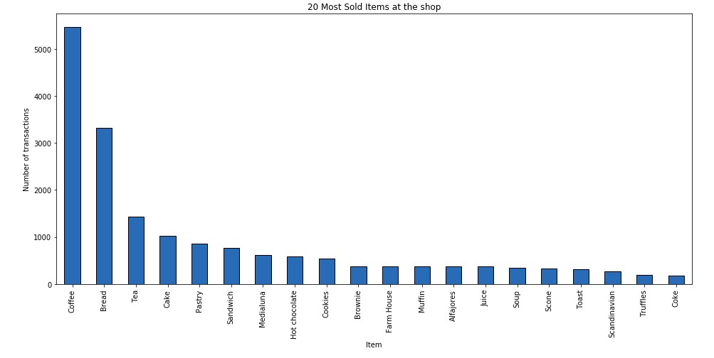
1. Around 48% of transactions contains `coffee`, 33% contains `bread`, 14% contains `tea` and 10% contains `cake`.
2. Together, coffee and bread are 9%, coffee, and tea 5%, coffee, and cake 5%, bread and tea 3%, bread and cake 2%, tea and cake 2%.

Installing & Importing Mlxtend library

To install mlxtend, just execute

`pip install mlxtend`

To install mlxtend using conda, use the following command:

`conda install mlxtend`

For using the apriori algorithm and extracting association rules, we will import apriori and association rules module from mlxtend.frequent patterns

#Importing required modules from mlxtend
from mlxtend.frequent_patterns import apriori
from mlxtend.frequent_patterns import association_rules

df.groupby(['Transaction', 'Item'])['Item'].count().unstack().fillna(0)

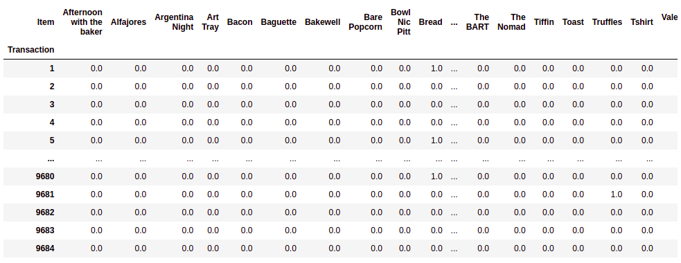
To use apriori algorithm and find out the relevant association rules, we need to convert the transactions into a user-item matrix such that each column is an item, and each value in the matrix is 1 if an item belongs to a transaction and 0 if an item does not belong to a transaction

Preprocessing Dataset for mining association rules using mlxtend

For applying the apriori algorithm from mlxtend library, we need to first convert this into a format where all the items are as columns and filled with 1 if an item is in the transaction and 0 otherwise.

#First step is to group it by transaction id and item to find item count in each transaction
df.groupby(['Transaction', 'Item'])['Item'].count()

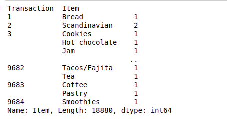
#To get each item in a separate column, we can use unstack
df.groupby(['Transaction', 'Item'])['Item'].count().unstack().head()

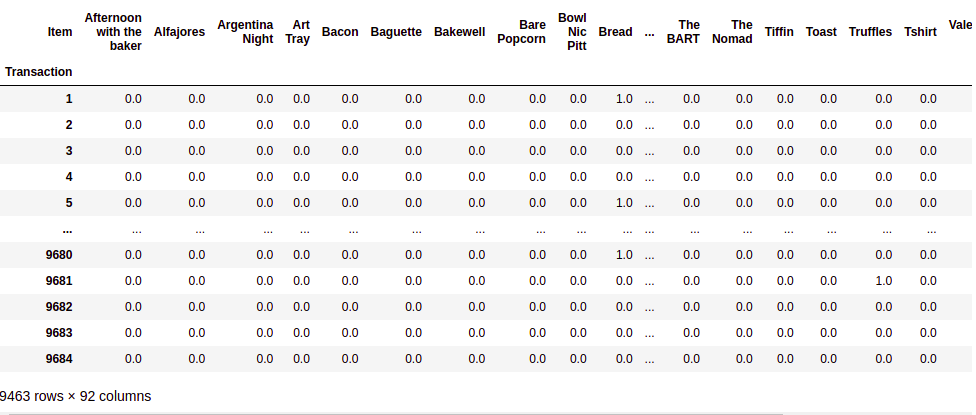
#Fill the missing values with 0 meaning that item is not there in a transaction
df.groupby(['Transaction', 'Item'])['Item'].count().unstack().fillna(0)

Source:- Author

#Finally you can store the result separately
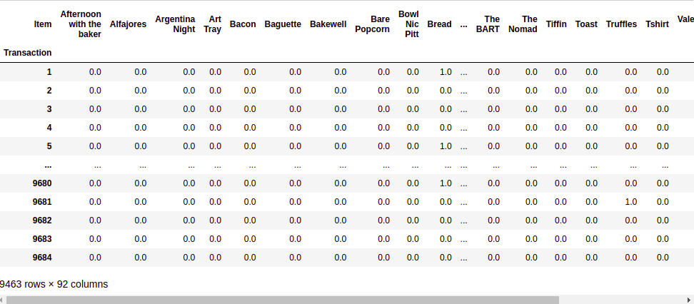
hot_encoded_df = df.groupby(['Transaction', 'Item'])['Item'].count().unstack().fillna(0)
hot_encoded_df

Source:- Author

In order to implement the Apriori algorithm, we don’t need the count of each item, for example, in transaction 2 we saw 2 Scandinavians but in order to identify an association, just a 1 or 0 is enough. We will define a function to say everything greater than 1 will be changed to 1

#Function to change all the values greater than or equal to 1 as just 1 and others to be 0
def encode_units(x):
    if x <= 0:
        return 0
    if x >= 1:
        return 1

#Applying the function to the encoded dataframe
hot_encoded_df = hot_encoded_df.applymap(encode_units)

Finding Frequent Itemsets with given support threshold using Apriori

We will use Apriori Algorithm to find the rules with a support threshold of 0.01 or 1%.

# using the 'apriori algorithm' with min_support=0.01 (1% of 9465)
# It means the item should be present in atleast 94 transaction out of 9465 
    transactions only when we considered that item in
# frequent itemset

frequent_itemsets = apriori(hot_encoded_df, min_support = 0.01, use_colnames = True)
frequent_itemsets

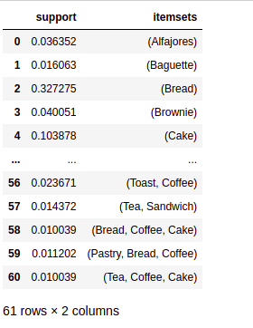
We see that the top support is for coffee and bread. Coffee and pastry and some other combinations, including coffee necessarily, were expected as coffee has the highest support.

We have used the apriori algorithm to find all items with top support values to prevent items that are uninteresting from a business point of view on account of being really rare from being removed. The next step is to measure the reliability of the inference made by the rule; we will check for confidence and lift for all these itemsets.

Finding top association rules with Lift & Confidence as the metrics

Once we have identified the frequent itemsets using the apriori algorithm, we can calculate parameters such as lift and confidence to see which of the rules can be established as the most important ones.

# now making the rules from frequent itemset generated above
rules = association_rules(frequent_itemsets, metric = "lift", min_threshold = 1)
rules.sort_values('confidence', ascending = False, inplace = True)
rules[['antecedents','consequents','support','confidence','lift']].head(5)

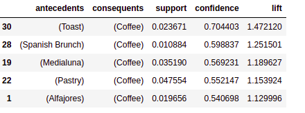
How to read the table?

Thanks for reading!

I hope that you have enjoyed the article. If you like it, share it with your friends also. Please feel free to comment if you have any thoughts that can improve my article writing. Here is my Linkedin profile if you want to connect with me.

You can read Previous Data Science Blog posts here if you want to read my previous blogs.

The media shown in this article is not owned by Analytics Vidhya and is used at the Author’s discretion.

kajal

Hi, I am Kajal Kumari. have completed my Master’s from IIT(ISM) Dhanbad in Computer Science & Engineering. As of now, I am working as Machine Learning Engineer in Hyderabad.
hope that you have enjoyed the article. If you like it, share it with your friends also. Please feel free to comment if you have any thoughts that can improve my article writing.

If you want to read my previous blogs, you can read Previous Data Science Blog posts here. Connect with me