Basic Introduction to Loss Functions

This article was published as a part of the Data Science Blogathon.

Introduction

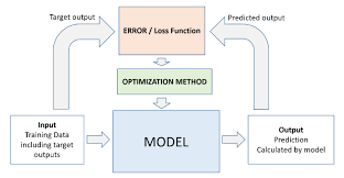
The loss function is as noteworthy to Machine Learning as the guide is important to a student. Just like a guide aids in improving the performance /efficiency of a student, similarly, loss functions are required to improve the output result of the model for better accuracy.

The loss function serves as the basis of modern machine learning. To put it simply, a loss function indicates how inaccurate the model is at determining the relationship between x and y. Loss functions serve as a gauge for how well your model can forecast the desired result.

Any statistical model utilizes loss functions, which provide a goal against which the model’s performance is evaluated.  The parameters that the model learns are then calculated by minimizing the selected loss function. The error (or simply the  “the loss”) between the output of our algorithms and the specified target value is calculated using loss functions.

The loss function assesses how your machine learning algorithm predicts the featured data set.

What is Loss Function

The loss function is the function that determines how far the algorithm’s current output is from what is desired. This is a technique for assessing how well our algorithm models the input. It can be divided into two categories. Both for regression and for classification

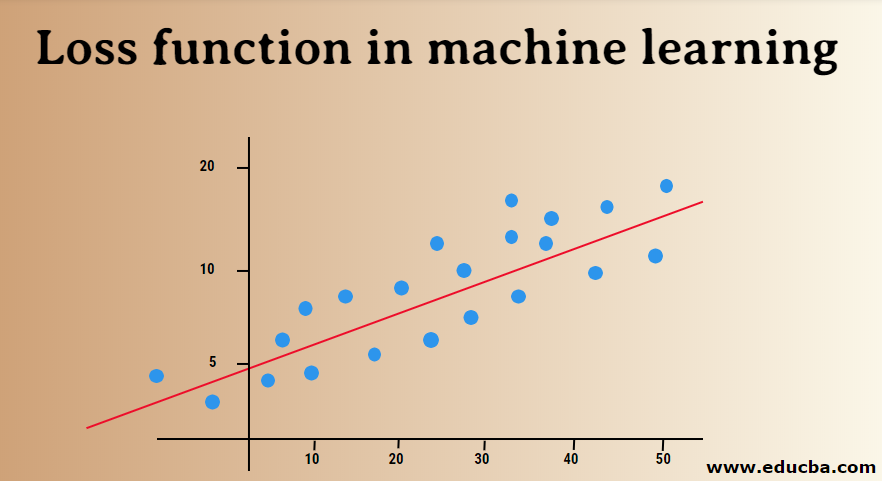
The loss function in machine learning distinguishes between the model’s projected output and the actual output for a single training example. In contrast, the cost function is the mean of the loss functions across all training examples.

Source:edcuba.com

Loss functions in neural networks aid in improving the model’s performance. They are typically employed to quantify a penalty the model imposes on its predictions, such as the prediction’s departure from the label representing the ground truth.

Loss functions and metrics varied slightly from one another as well. Loss functions can provide data on the effectiveness of our model, but they may not be directly relevant or simple to understand for humans. Metrics are useful in this situation. Even though they may not be the best options for loss functions since they may not be differentiable, metrics like accuracy are considerably more useful for people to comprehend how well a neural network performs.

Regarding the problems we encounter in the actual world, loss functions can be broadly divided into classification and regression. Our task in classification problems is to predict the respective probability of each class that the challenge involves. The goal of regression, on the other hand, is to forecast the continuous value for a given collection of independent features to the learning algorithm.

Several Regression Loss Functions

The regression includes making a particular, continuous value prediction. Regression examples include estimating home prices and forecasting stock prices because they both aim to create models that can forecast real-valued quantities.

Mean Absolute Error

The total absolute difference between the actual and projected variables is calculated using MAE. The average size of mistakes in a group of projected values is thus measured. While the absolute error is much more resistant to outliers, the mean square error is simpler to address. Outlier values are ones that significantly differ from other reported data points.

If the prediction and the ground truth were identical, the MAE would be zero, which it never is. Given that you wish to reduce the inaccuracy in your predictions, a regression problem might benefit from using this straightforward loss function as one of your measurements.

MAE averages out the absolute disparities between the actual and anticipated values. When a data point x_i and its anticipated value y_i are considered, where n is the total number of data points in the collection

The mean absolute error ( Mathematical formula) is defined as follows:

Python Implementation

import numpy as np

def mean_absolute_error(act, pred):

diff = pred - act

abs_diff = np.absolute(diff)

mean_diff = abs_diff.mean()

return mean_diff

act = np.array([1.1,2,1.7])

pred = np.array([1,1.7,1.5])

mean_absolute_error(act,pred)

Mean Squared Error

The average squared difference between the actual and model-predicted values is measured by MSE(L2 error). A single number that corresponds to a range of values is the output. Our goal is to lower MSE to increase the model’s accuracy.

The mean squared error is the average of the squared discrepancies between the actual and anticipated values. Models trained with mean squared error have fewer outliers or at least less severe outliers than models trained with mean absolute error because mean squared error prioritizes a large number of little errors over a few large errors.

The mathematical formula is defined below:

Source: Medium.com

Python Implementation

import numpy as np

def mean_squared_error(act, pred):

   diff = pred - act
   differences_squared = diff ** 2
   mean_diff = differences_squared.mean()
   
   return mean_diff

act = np.array([1.1,2,1.7])
pred = np.array([1,1.7,1.5])

print(mean_squared_error(act,pred))

Mean Bias Error

The mean bias in the model is calculated using Mean Bias Error. In a word, bias is the over- or underestimation of a parameter.

Mean Bias Error uses the actual, not the absolute, difference between the target and the forecasted result.

Python Implementation

# Mean Bias Error
 
def mbe( y, y_pred ) :
return np.sum( y - y_pred ) / np.size( y )

Mean Squared Logarithmic Error Loss (MSLE)

The MSLE calculates the ratio of the actual value to the expected value. The error curve becomes asymmetric as a result. Only the percentage difference between the actual and anticipated values is important to MSLE. When we want to forecast house sales or bakery sales prices and the continuous data, it can be a viable option for a loss function.

Some of the Loss Functions for Classification

Determining a discrete class output is a challenge in classification tasks. It entails categorizing the dataset into distinct classes depending on various factors so that a brand-new record can be added to one of the classes.

Binary Cross-Entropy

This loss function serves as the default one for binary classification issues. A classification model’s effectiveness is calculated using the cross-entropy loss, which outputs a probability value between 0 and 1. The cross-entropy loss grows as the anticipated probability value deviates from the actual label.

Python Implementation

# calculate binary cross entropy
def binary_cross_entropy(actual, predicted):
	sum_score = 0.0
	for i in range(len(actual)):
		sum_score += actual[i] * log(1e-15 + predicted[i]
	mean_sum_score = 1.0 / len(actual) * sum_score
	return -mean_sum_score

Hinge loss

Cross-entropy, initially created to be utilized with a support vector machine algorithm, can be replaced by hinge loss. The classification issue benefits from hinge loss the most because the target values fall into the range of -1,1. If there is a change in sign between the actual and anticipated numbers, it enables the assignment of greater error. Consequently, it performs better than cross-entropy.

Python Implementation

# Hinge Loss
def hinge(y, y_pred):
l = 0
size = np.size(y)
for i in range(size):
l = l + max(0, 1 - y[i] * y_pred[i])
return l / size

Kullback Leibler Divergence Loss (KL Loss)

A distribution’s Kullback Leibler Divergence Loss gauges how different it is from a standard distribution. When the Kullback Leibler Divergence Loss is 0, the probability distributions are the same for both cases.

Squared hinge loss

In addition to hinge loss, that only computes the hinge loss score’s square. It makes it easier to work numerically and reduces the error function. It identifies the categorization border that establishes the largest possible difference between data points of different classes.

Log Loss

Assesses how accurately a model gives probabilities for different outcomes, especially in tasks where you categorize things.

Some of the Loss Functions for Multi-class Classification

Multi-class classifications are Predictive
models where more than two classes are being allotted.

Multi-class Cross-Entropy

In this instance, the target values are 0 to n, or 0 to 1, 2, 3, and n. To achieve the highest level of accuracy, a score is calculated by averaging the differences between actual and anticipated probability values.

Multi-class Sparse Cross-Entropy

Multi-class cross-entropy has difficulty handling many data points due to one hot encoding operation. This issue is resolved by sparse cross-entropy, which calculates error without using one-hot encoding.

Conclusion

So in this article, we studied loss functions in an introductory manner. We saw how loss functions play an important role in modern-day machine learning problems. We also saw how the model’s performance depends on its loss function and how it helps optimize the output.

Some of the following points we covered in this article

1. We studied loss function and its significance in machine learning
2. We also studied the working of the loss function and its role in getting optimized output from the respective machine Learning model
3. We also studied various types of loss functions used in regression problems
4. We also studied various types of loss functions used in classification problems as well as in multi-class classification problems
5. We also covered python implementation of some of the common loss functions being employed in both regression and classification problems
6. We studied about mean squared loss and its python implementation as well as its mathematical formula
7. Basically, We covered  common loss functions for regression as well classification(binary and multiclass) along with their explanation and python implementation

Frequently Asked Questions

I hope you liked my article; Please share it in the comments below.

My name is Pranshu Sharma, and I am a Data Science Enthusiast. Thank you so much for taking your precious time to read this blog. Feel free to point out any mistake(I’m a learner, after all) and provide respective feedback or leave a comment.

Feedback:Email: [email protected]

The media shown in this article is not owned by Analytics Vidhya and is used at the Author’s discretion.

Pranshu Sharma

Aspiring Data Scientist | M.TECH, CSE at NIT DURGAPUR