This article was published as a part of the Data Science Blogathon.
Introduction
Template matching is a high-level computer vision approach that detects image portions that match a predetermined template. Advanced template matching algorithms detect template occurrences regardless of orientation or local brightness.
In medical image analysis, invariant characteristics or innovative applications are commonly used as object identification domains such as vehicle tracking, robotics, and manufacturing.
Template Matching approaches are versatile and simple to apply, making them one of the most used ways of object localization. Their utility is restricted mostly by computer capacity, as identifying large and complicated templates can be time-consuming.

- It is a way of searching for and locating a template within a larger image.
- The goal is to discover identical portions of an image that match a template we provide based on a threshold.
- The threshold determines how well we want to recognize the template in the original image.
- For example, if we are using face recognition and want to detect a person’s eyes, we can use a random image of an eye as the template and search for the source (the face of a person).
- In this scenario, because “eyes” vary so much from person to person, even if we set the threshold to 50% (0.5), the eye will be recognized.
Working Function
- Simply slide the template picture over the input image (as in 2D convolution)
- The template picture and the piece of input image beneath it are compared.
- The acquired result is compared to the threshold.
- If the result exceeds the threshold, the section is marked as detected.
- The first parameter in the function cv2.matchTemplate (image, template,cv2.TM_CCOEFF_NORMED) is the main image, the second parameter is the template to be matched, and the third parameter is the matching technique.
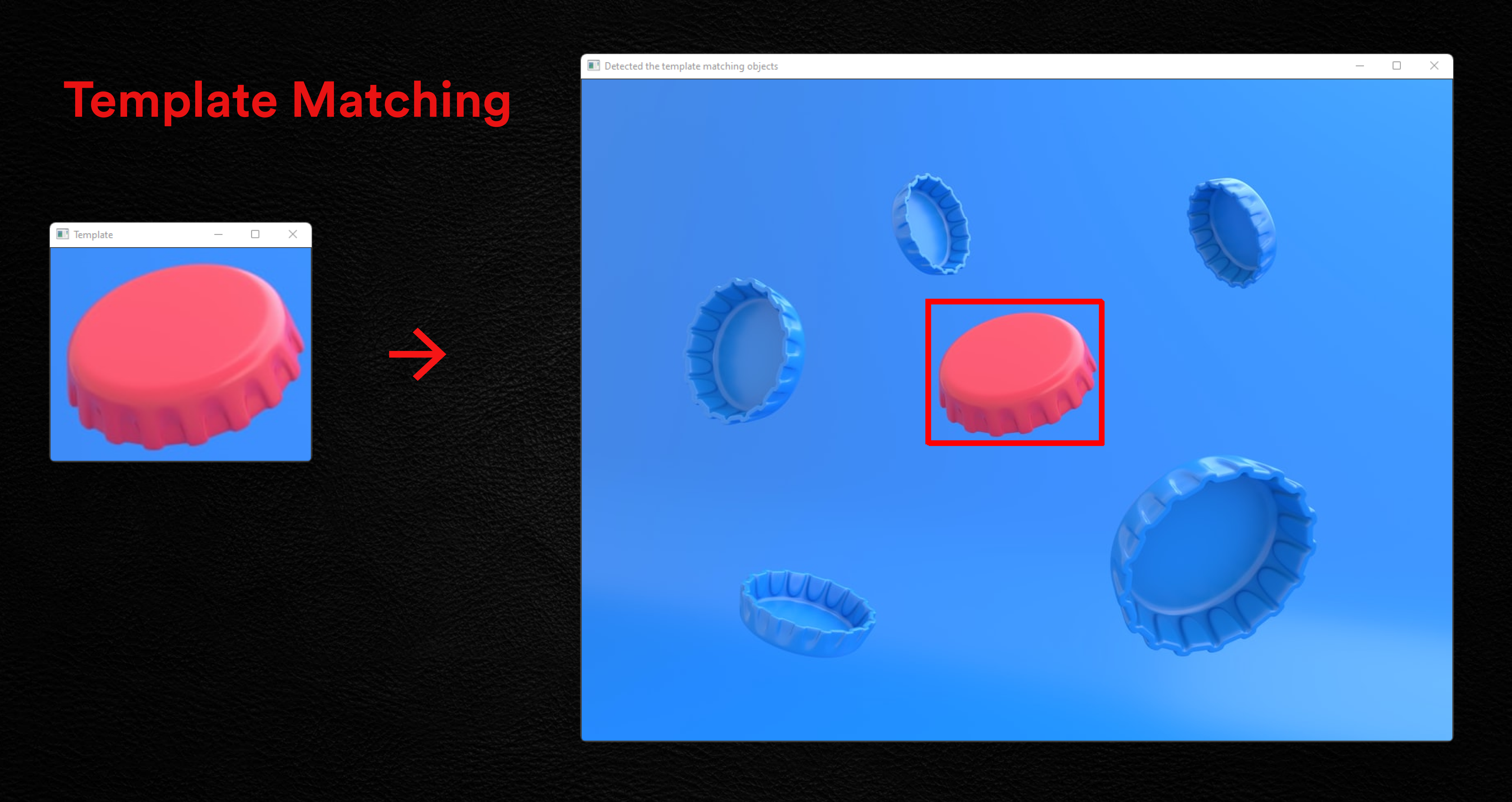
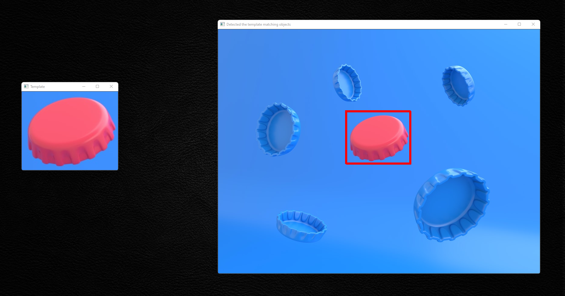
Let us first define template matching. It is a method for locating a reference image (or a template image) within a source image. In its most basic form, the algorithm compares the template for each source image region, one pixel at a time. This is referred to as cross-correlation. The result of this procedure is another image with a pixel value that corresponds to how similar the template image was to the source image when it was inserted at that pixel location.
Let’s look at an image of a Metal Bottle cap to see how this works. Assume that we are interested in the Red Metal Bottle Cap.
Let’s Code
Let us see its implementation in Python! But first, we have to import the following libraries:
import cv2
import numpy as np
Let’s load a source image and convert your RGB source image to greyscale (its binarized form might also work). Color photos can be used for template matching, although greyscale or binarized images are easier to use.
.png)
To conduct Template matching in the above image, first, we have to load the template image
.png)
template = cv2.imread(r"template_image_path")
w, h = template.shape[::-1]
After storing the template’s width and height in w and h, we initialize a variable discovered to keep track of the region and scale of the image with the best match. Use the template-matching function to detect the template in the Input source Image,
res = cv2.matchTemplate(gray, template, cv2.TM_CCOEFF_NORMED)
After that, set the threshold for the desired output
threshold = 0.90
loc = np.where(res >= threshold)
Draw the rectangle in template matched objects
for pt in zip(*loc[::-1]):
    cv2.rectangle(img, pt, (pt[0] + w, pt[1] + h), (0, 0, 255),1)
Show the Source Image with marked template region
cv2.imshow('Detected the template matching objects', img)
cv2.imshow('Template', template)
cv2.waitKey()
cv2.destroyAllWindows

We can utilize multiscaling to avoid the problem caused by the various sizes of the template and original image.
Multiscaling- New Template Matching Approach
If the dimensions of your template do not match the dimensions of the region in the image you want to match, this does not preclude you from using template matching.
The Multi scaling procedure is as follows:
Loop through the input image at various scales. Using cv2.matchTemplate, apply template matching and keep track of the match with the highest correlation coefficient (along with the x and y-coordinates of the region with the largest correlation coefficient). After cycling through all scales, select the zone with the highest correlation coefficient as your “matched” region.
import cv2

import imutils

import numpy as np

img_rgb = cv2.imread('mainimage.jpg')

img_gray = cv2.cvtColor(img_rgb, cv2.COLOR_BGR2GRAY)

template = cv2.imread('template', 0)

w, h = template.shape[::-1]

resize = imutils.resize(img_gray, width=int(img_gray.shape[0]), height=int(img_gray.shape[1]*scale)

if resized.shape[0] < h or resized.shape[1] < w:

break

found=(maxVal, maxLoc, r)

(__, maxLoc, r)=found

(startX, startY)=(int(maxLoc[0]*r), int maxLoc[1]*r)

(finalX, finalY)=(int((maxLoc[0]+tw)*r), int(maxLoc[1]+tH)*r)

cv2.rectangle(image, (startX, startY),(finalX, finalY), (255, 0, 255), 2)

cv2.imshow("Image", image)

cv2.waitKey(0)
The following is a step-by-step explanation of the above code:
We initialize a variable discovered to keep track of the region and scale of the image with the best match after recording the width and height of the template in w and r. Then, using the np.linspace function, we begin looping across the image’s numerous scales. This function takes three arguments: the starting and ending values and the number of equal chunk slices between them. In this example, we’ll start with 100% of the original image size and work down to 20% of the original size in 20 equally sized percent chunks.
We next resize the image to the current scale and compute the ratio of the previous width to the new width – as you’ll see later, this ratio is critical. We verify that the supplied image is larger than our template matching. If the template is larger, our cv2.matchTemplate call will fail. Therefore, we just exit the loop in this instance. We can now apply template matching to our scaled image:
Our correlation result is passed to the cv2.minMaxLoc function, which returns a 4-tuple containing the minimum correlation value, the maximum correlation value, the (x, y)-coordinate of the minimum value, and the (x, y)-coordinate of the maximum value, respectively.
Because we only want the maximum value and (x, y)-coordinate, we save the maximums and reject the minimums. Following that, we inspect the matched image regions at each scale iteration. Then, we update our discovered variable to keep track of the largest correlation value discovered thus far, the (x, y)-coordinate of the maximum value, and the ratio of the original image width to the current, enlarged image width.
After looping through all picture scales, we extract our discovered variable and compute the starting and ending (x, y)-coordinates of our bounding box.
Conclusion
This article demonstrated how we can use Image Processing to aid with Object Detection and Recognition. We could detect all the miniature flower bouquets using only one of the flower bouquets as a template utilizing the examples provided.
Template matching can be utilized as a pipeline in the detection of objects for machine learning and deep learning models.
Key Takeaways:
- The orientation of the reference pattern picture must be preserved in pattern occurrences (template).
- As a result, it does not function for rotated or scaled versions of the template because a change in the shape/size/shear, etc., of the object about the template, would result in a false match.
- Because the process is time-consuming, the method is inefficient when calculating the pattern correlation image for medium to large photos.
Keep an eye out for more articles!
The media shown in this article is not owned by Analytics Vidhya and is used at the Author’s discretion.


