This article was published as a part of the Data Science Blogathon.
Introduction
During the 20th century, movies were released in Theatres. It was a time when there was no Internet, so people relied on word of mouth to decide which movie to watch. Also, the movie options were limited. Only a few movies were released each week. However, much content has been published daily with the advent of digital media and OTT platforms in the last decade. Much content is available to watch on social media or OTT platforms. So, it becomes essential for someone to do some due diligence before watching a movie. Most of these OTT platforms give personalised recommendations to users.
Suppose you get a recommendation of 100 movies, and you shortlist a single movie to watch but are still reluctant about whether it is worth your time. So, you may watch the trailer, but the trailers are always good and do not give a clear idea about the movie. Then, you might prefer to check IMDB. You may check the ratings, plot, cast, etc. Sometimes, you may read a few reviews to understand the user’s perception of that movie and may end up knowing the spoiler.
Is there a way to analyse the reviews without knowing the spoiler?
Text analysis using NLP (Natural Language Processing) is a way to identify, extract and understand the main mood or prejudice of the reviewer. Now that IMDB rating data is available, you can analyse the ratings, do time trend analysis, or dig deeper into the reviews to extract interesting perspectives.
NLP Problem Statement
In my previous article, we saw how scrapy and selenium extract a particular title’s reviews from the IMDB website. This article will use the same data, i.e., reviews extracted from the movie “Harry Potter and the Sorcerer’s Stone.” We will do an in-depth analysis using the NLP of a movie to understand several trends.
Data Download for NLP
Using the steps in the above article, scrape all the IMDB reviews for the movie “Harry Potter and the Sorcerer’s Stone.” It should take approximately 5 minutes (faster if you have a good Internet speed) for the entire scraping to be complete. An Excel file will be created if you follow the scraping instructions as per the article.
Let us understand the columns of that file:
- Review_Date: The date the review was written
- Author: The name of the reviewer
- Rating: The rating given by the author (scale of 1 to 10)
- Review_Title: The summary given by the reviewer
- Review: The entire opinion of the reviewer about the title
- Review_Url: The URL of the review.
Import Libraries using NLP
Let us load all the relevant libraries for our analysis
import pandas as pd
import numpy as np
import syllables
from nltk.stem import WordNetLemmatizer
from nltk import tokenize,ngrams
from nltk.corpus import stopwords
import re
import textstat
import itertools
import collections
import matplotlib.pyplot as plt
from sklearn.feature_extraction.text import CountVectorizer
from wordcloud import WordCloud, STOPWORDS
Load the above dataset
df = pd.read_excel('../IMDB_Reviews/Harry_Potter_1_reviews.xlsx')
Text Processing using NLP
Since we will focus on dissecting the reviews to perform text analysis, we must do some text preprocessing.
We will apply the below string cleaning steps.
- Remove non-alphanumerics
- Remove URLs
- Remove line breaks
- Replace more than one whitespace with a single space
def clean_text(a):
    a_replaced = re.sub('[^A-Za-z0-9]+', ' ', a)
    a_replaced = re.sub(r'w+:/{2}[dw-]+(.[dw-]+)*(?:(?:/[^s/]*))*', '', a_replaced)
    a_replaced = re.sub('n', ' ', a_replaced)
    a_replaced = re.sub(' +', ' ', a_replaced)
    return a_replaced
Feature Engineering
1. Create Feature: Review_Word count
This represents the total word count across each review.
df['Review_Words'] = df['Review'].apply(lambda x : len( x.split()) )
2. Create Feature: Review_Date_Cleaned column
Here, we will convert the Review_Date column into a pandas datetime format.
df['Review_Date_Cleaned'] = pd.to_datetime(df['Review_Date']).dt.date
3. Create Feature: Syllables
Syllables are phonological “building blocks” for each word. Syllabic writing began hundreds of years before the first letters. The oldest syllable is found on clay tablets from around 2800 BC in the Sumerian city of Ur. This shift from pictograms to syllables is considered the most important evolution in writing history.
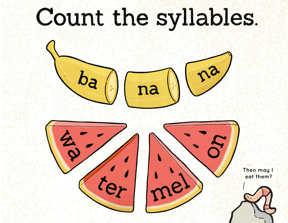
Image Source: https://en.m.termwiki.com/EN:Syllable
In the above image, we can see that the word banana has 3 syllables, and the word watermelon has 4 syllables.
We will create a column to calculate the Total_Syllables for each review. Additionally, we will also calculate Average_Syllables for each review. This will be calculated as Total_Syllables/Total_Words.
e.g. sentence = ‘Banana and watermelon are both fruits’
The above sentence has total syllables =12 and a total words = 6.
So the Average_Syllables will be 12/6 = 2.
df['Total_Syllables'] = df['Review'].apply(lambda x : syllables.estimate(x))
df['Average_Syllables'] = df['Total_Syllables']/df['Review_Words']
4. Create Feature: Flesch Reading Ease
Created for the US Navy in 1975, it helps determine how easy it is to read a particular written text. Formula :
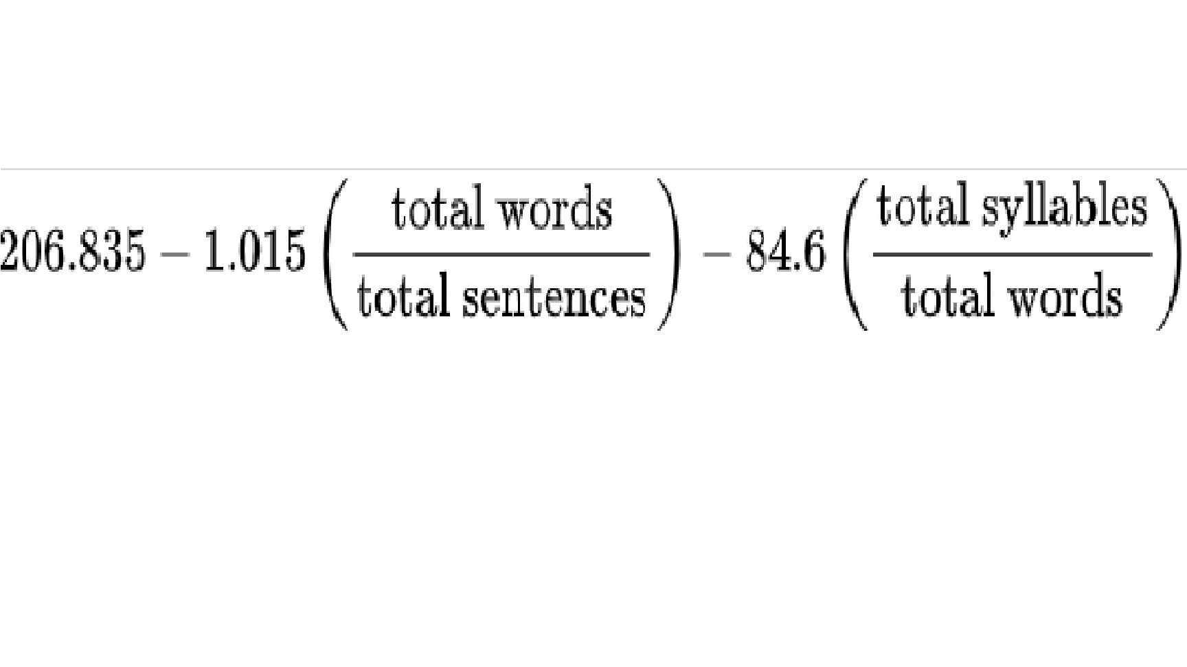
Image Source https://wikimedia.org/api/rest_v1/media/math/render/svg/bd4916e193d2f96fa3b74ee258aaa6fe242e110e :
The score created using the above formula is categorised as below:
| Score | School level | Notes |
|---|---|---|
| 100.00-90.00 | 5th grade | Very easy to read. Easily understood by an average 11-year-old student. |
| 90.0–80.0 | 6th grade | Easy to read. Conversational English for consumers. |
| 80.0–70.0 | 7th grade | Fairly easy to read. |
| 70.0–60.0 | 8th & 9th grade | Plain English. Easily understood by 13- to 15-year-old students. |
| 60.0–50.0 | 10th to 12th grade | Fairly hard to read. |
| 50.0–30.0 | College | Hard to read. |
| 30.0–0.0 | College Graduate | Very hard to read. Best understood by university graduates. |
The highest score possible is 121.22
However, some complicated sentences can even have a negative score.
e.g. of, a negative flesh reading score from the corpus.
df['flesch_reading_ease'] = df['Review'].apply(lambda x : textstat.flesch_reading_ease(x) )
# Example of a negative readability example
a = df.sort_values(by='flesch_reading_ease').head().iloc[1]
print(a['flesch_reading_ease'])
print()
print(a['Review'])
Output
Score: -91.6

I have to say I am disappointed in the reviews it makes me wonder if those that have seen it saw the same movie my husband(who is 32) and myself (24) have already seen twice I could not have imagined a better cast when I first read the first book right off the bat I knew who should (if they made a movie) play Snape Alan Rickman did a great job as did the child stars who play Harry,Hermione, and Ron I can not wait for the second one to come out, and can not wait for the new book Chris Columbus did a wonderful job, and except for a few parts the FX are great and the parts that are cut out are not that big of a deal that they mess up the story line, as for someone saying as long as your are between the ages of 3 and 13 you will enjoy it that is hogwash this is a movie for the entire family and I know I will be going to see it again while it is in theaters and will buy it when it comes out on DVD.
The above review is fairly complex to read. Hence, the negative score makes sense.
5. Create Feature: review lemma
The entire review may contain a lot of words. Some words are more frequently used in English, like ‘the’, ‘a’, ‘of’, etc. Such words are known as stopwords and do not carry much significance in our analysis.
Also, each word can be converted into its root form to reduce the vocabulary size.
e.g. the root word for “studying”, “studies”, and “study” is “study”. This root word is known as a lemma. The root word produced after lemmatization has a meaning in English vocabulary.
w_tokenizer = tokenize.WhitespaceTokenizer()
lemmatizer = WordNetLemmatizer()
def lemmatize_text(text):
    return [lemmatizer.lemmatize(w) for w in w_tokenizer.tokenize(clean_text(text.lower())) if w not in stopwords.words('english')]
df['review_lemmas'] = df['Review'].apply(lambda x : lemmatize_text(x))
The above step might take a couple of minutes to run. Be patient.
6. Create Feature: Time Period
Let us take a quick look at the Review published year.
pd.to_datetime(df['Review_Date']).dt.year.value_counts()
Output
2001    676
2002    358
2020    135
2021     92
2022     79
2003     66
2005     59
2019     54
2004     52
2018     48
2007     40
2006     37
2008     33
2016     30
2009     28
2013     25
2015     25
2011     25
2010     20
2012     20
2014     19
2017     19
Name: Review_Date, dtype: int64
It seems like 676 reviews were written in 2001 itself. It makes sense; people usually express their sentiments or opinions when watching the movie. Given that the movie was released in 2001, most reviews are usually from that year. We will divide the time window into 3 periods so that each period has a substantial number of reviews we can perform analysis on.
Period 1: All reviews written in 2001
Period 2: All reviews written between 2002 and 2011
Period 1: All reviews are written post-2011
df['Period'] = np.where(pd.to_datetime(df['Review_Date']).dt.year>=2012,'c. Post 2011','Other')
df['Period'] = np.where(pd.to_datetime(df['Review_Date']).dt.year<2012,'b. Btn 2002 and 2011',df['Period'])
df['Period'] = np.where(pd.to_datetime(df['Review_Date']).dt.year<2002,'a. During 2001',df['Period'])
df['Period'].value_counts()
Output:
b. Btn 2002 and 2011    718
a. During 2001          676
c. Post 2011            546
Name: Period, dtype: int64
EDA
1. EDA: Rating
Now let’s take a quick look at the rating trend.
print(df['Rating'].isnull().sum())
print(df['Rating'].agg(['mean','median','count']).round(2))
df['Rating'].value_counts().reset_index().sort_values(by='index').plot.barh(x='index', y='Rating', color="purple")
Output:
353
mean         7.71
median       8.00
count     1587.00
Name: Rating, dtype: float64
Insights:
- 353 reviews do not have a rating.
- The remaining reviews’ mean rating is 7.7, and the median is 8.
- a lot of reviews have a rating of 10.
- A higher review count is observed when rating>=7.
Let us look at how the rating span across the Time Period
df.groupby('Period')['Rating'].agg(['min','mean','median','max','count']).round(2)
Output
| min | mean | median | max | count | |
|---|---|---|---|---|---|
| Period | |||||
| a. During 2001 | 1.0 | 7.58 | 8.0 | 10.0 | 507 |
| b. Btn 2002 and 2011 | 1.0 | 7.31 | 8.0 | 10.0 | 552 |
| c. Post 2011 | 1.0 | 8.25 | 8.0 | 10.0 | 528 |
The min, median, and max values of Rating are the same across all 3 Periods.
However, if we look at the mean value, we can see that the mean rating was higher in 2001; it decreased between 2002 and 2011. However, post-2011, the mean rating increased beyond 8. This means that the people who posted reviews post-2011 found the movie good and rated it above 8. No spoilers so far. Just an indication that the movie is worth watching.
Let us also look at the days of the week the review is posted.
df['Review_Day'] = pd.to_datetime(df['Review_Date']).dt.day_name()
df['Review_Day_no'] = pd.to_datetime(df['Review_Date']).dt.dayofweek
# a = df['Review_Day_no'].value_counts().reset_index().sort_values(by='index')
a = df.groupby(['Review_Day_no','Review_Day']).Review.count().reset_index()
a.plot.barh(x='Review_Day_no', y='Review', color="purple")
Here, 0 represents Monday, and 6 represents Sunday.
Insights:
- We can see that Saturday is when most of the reviews are posted.
- On a similar note, Tuesday is when the review count is minimal.
- An interesting trend is that the review count increases across the week i.e. it was lowest on Tuesday, increased on Wednesday, and kept on increasing till Saturday.
Let us look at the Day wise trend across time.
df.groupby('Period')['Review_Day_no'].agg(['count'])
a = df.pivot_table(index='Review_Day_no',columns='Period',values='Review',aggfunc='count',margins=True)
a = (a*100).div(a.loc['All']).round(2)
a
Output
| Period | a. During 2001 | b. Btn 2002 and 2011 | c. Post 2011 | All |
|---|---|---|---|---|
| Review_Day_no | ||||
| 0 | 19.53 | 14.35 | 13.37 | 15.88 |
| 1 | 8.14 | 13.93 | 13.37 | 11.75 |
| 2 | 9.02 | 14.62 | 14.10 | 12.53 |
| 3 | 8.28 | 13.79 | 17.58 | 12.94 |
| 4 | 14.94 | 11.28 | 15.20 | 13.66 |
| 5 | 19.82 | 17.55 | 14.65 | 17.53 |
| 6 | 20.27 | 14.48 | 11.72 | 15.72 |
| All | 100.00 | 100.00 | 100.00 | 100.00 |
Here, each column is shown as a percentage distribution.
Interpretation: If there were 100 reviews posted During 2001, approximately 19.53% were posted on Monday, 8.14% were posted on Tuesday, and so on.
Insights:
- During 2001, most of the reviews were posted on Weekends and Monday. This makes sense because back in 2001, we did not have OTT platforms, so people used to watch movies in theatres.
- Since most people watch a movie in the theatre over a weekend, so most of the reviews are posted during that time.
- Between 2001 and 2011, people had access to TV, DVD, and home entertainment. So, we see the reviews posted across all the days.
- Post-2011, we saw the advent of Netflix, and several other OTT players started popping up in the last 5 years. Now, people can watch a movie at the tip of their fingertips (even on a mobile device). So, the reviews are posted across all the days more evenly now.
This is an exciting trend.
2. EDA: Review_Words
Let us look at how many reviews have just a single word.
print(df[df['Review_Words']==1].shape)
Output:
(1, 15)
Ahh, only a single review; let’s look at the actual review.
df[df['Review_Words']==1]['Review'].iloc[0]
Output:
'👌🏻👌🏻👌🏻👌🏻👌🏻👌🏻👌🏻👌🏻👌🏻👌🏻👌🏻👌🏻👌🏻👌🏻👌🏻👌🏻👌🏻👌🏻👌🏻👌🏻👌🏻'
It contains only a string of emojis.
Let us look at the word count across the time
df.groupby('Period')['Review_Words'].agg(['min','mean','median','max','count']).round(2)
Output:
| min | mean | median | max | count | |
|---|---|---|---|---|---|
| Period | |||||
| a. During 2001 | 23 | 233.66 | 177.0 | 1344 | 676 |
| b. Btn 2002 and 2011 | 37 | 232.87 | 167.5 | 1581 | 718 |
| c. Post 2011 | 1 | 171.49 | 111.0 | 1470 | 546 |
Insights:
- The median and mean values of Review_Words are decreasing over time.
- It’s interesting to see that the mean rating decreased from ~233 to ~171, which is an approximate 26% reduction in the review length.
- It is an indicator that people have been more succinct in recent years.
3. EDA: Are people using more numbers in recent times?
Let us create a dataframe that stores the start of the word and calculates the relative distribution.
We will create a column Start_Vowel using the below rules:
- If the 1st letter belongs to the set [‘a’, ‘e’, ‘i’ ,’o’, ‘u’], we will tag it as a vowel.
- If the 1st letter is a number, we will tag it as a number.
- If the above 2 conditions are not satisfied, we will tag it as a consonant.
Note: We can apply the above conditions as we have used only alphanumerics in the review_lemmas column.
full_start_letter_df = pd.DataFrame()
for period in sorted(df['Period'].unique()):
    curr_lemmatized_tokens = list(df[df['Period']==period]['review_lemmas'])
    curr_token_list = list(itertools.chain(*curr_lemmatized_tokens))
    start_letter = [i[0] for i in curr_token_list]
    start_letter_df = (pd.DataFrame(start_letter)[0].value_counts(1)*100).reset_index().sort_values(by='index')
    start_letter_df[0] = start_letter_df[0]
    start_letter_df.columns = ['letter',period]
    start_letter_df['Start_Letter'] = np.where(start_letter_df['letter'].isin(['a','e','i','o','u']),'a. Vowel',
                                                  np.where(start_letter_df['letter'].isin(['0','1','2','3','4','5','6','7','8','9']),'c. Number',
                                                       'b. Consonant')
                                              )
    start_letter_df = start_letter_df.groupby('Start_Letter')[period].sum().reset_index()
    start_letter_df.columns = ['Start_Letter',period]
    start_letter_df[period] = start_letter_df[period].apply(lambda x : np.round(x,2))
    try:
        full_start_letter_df = full_start_letter_df.merge(start_letter_df)
    except:
        full_start_letter_df = start_letter_df
print(full_start_letter_df.shape)
full_start_letter_df
Output
(3, 4)
| Start_Letter | a. During 2001 | b. Btn 2002 and 2011 | c. Post 2011 | |
|---|---|---|---|---|
| 0 | a. Vowel | 15.73 | 15.46 | 15.43 |
| 1 | b. Consonant | 82.84 | 83.22 | 83.07 |
| 2 | c. Number | 1.43 | 1.32 | 1.50 |
Here, each column is represented as a percentage. i.e. In 2001 – 15.73% of the words began with the vowel and so on.
Insights:
- We can see that the words starting with Vowels are reduced.
- Also, we can see that in Post 2011, reviews contain more numbers.
4. EDA: Average_Syllables
Let us look at the average_syllables trend across the time
df.groupby('Period')['Average_Syllables'].agg(['mean','median','count']).round(2)
Output:
| mean | median | count | |
|---|---|---|---|
| Period | |||
| a. During 2001 | 1.46 | 1.46 | 676 |
| b. Btn 2002 and 2011 | 1.45 | 1.45 | 718 |
| c. Post 2011 | 1.50 | 1.50 | 546 |
Insights:
- If we look at the mean values across time, we see a slight decrease from Period 1 to Period 2.
- However, there was a good increase in Period 3 (1.45 to 1.50). It means that the recent reviews are using slightly complex words.
Let’s validate the same using the flesh readability score.
5. EDA: flesch readability score
Let us look at the flesch readability score trend across time
display(df.groupby('Rating')['flesch_reading_ease'].agg(['mean','median','count']).round(2))
df.groupby('Period')['flesch_reading_ease'].agg(['mean','median','count']).round(2)
Output
| mean | median | count | |
|---|---|---|---|
| Rating | |||
| 1.0 | 77.65 | 78.79 | 71 |
| 2.0 | 73.39 | 72.70 | 23 |
| 3.0 | 74.36 | 74.69 | 35 |
| 4.0 | 73.65 | 74.19 | 41 |
| 5.0 | 74.99 | 74.53 | 81 |
| 6.0 | 72.15 | 71.99 | 101 |
| 7.0 | 70.57 | 71.95 | 229 |
| 8.0 | 70.76 | 72.89 | 286 |
| 9.0 | 74.86 | 75.78 | 256 |
| 10.0 | 76.28 | 78.08 | 464 |
| mean | median | count | |
|---|---|---|---|
| Period | |||
| a. During 2001 | 74.99 | 75.78 | 676 |
| b. Btn 2002 and 2011 | 74.71 | 75.22 | 718 |
| c. Post 2011 | 71.57 | 73.17 | 546 |
Insights:
- If we look at the analysis, we see that reviews having ratings of 1 or 10 have higher flesh readability scores. This means that these reviews are easy to understand.
- It makes sense when people rate the highest they talk about the positive highlights, and they rate the lowest when they express their dissatisfaction and opinion about the movie.
- If we look at the mean values across time, we see a slight decrease from Period 1 to Period 2.
- However, there was a good decrease in Period 3 (74.7 to 71.5), Which means that the recent reviews are slightly more complicated to read and use more complex words.
- This is something we saw in the Average_Syllables trend as well.
6. EDA: Looking at the top words mentioned in the reviews
lemmatized_tokens = list(df['review_lemmas'])
%matplotlib inline
token_list = list(itertools.chain(*lemmatized_tokens))
counts_no = collections.Counter(token_list)
# counts_no = collections.Counter(ngrams(token_list, 1))
clean_reviews = pd.DataFrame(counts_no.most_common(30), columns=['words', 'count'])
fig, ax = plt.subplots(figsize=(12, 8))
clean_reviews.sort_values(by='count').plot.barh(x='words', y='count', ax=ax, color="purple")
ax.set_title("Most Frequently used words in Reviews")
plt.show()
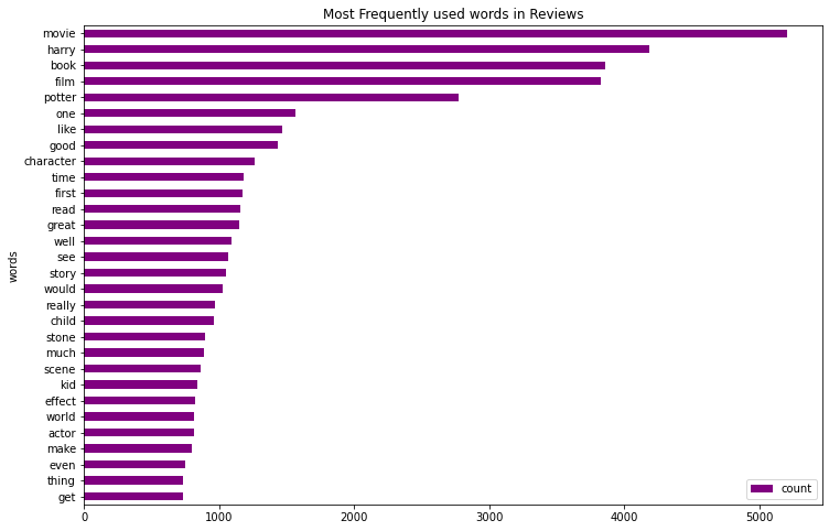
The most popular word is “movie”, followed by “harry” and so on. This gives good insight.
Let’s look at the top 10 words for each of the time periods.
for period in sorted(df['Period'].unique()):
    lemmatized_tokens = list(df[df['Period']==period]['review_lemmas'])
    token_list = list(itertools.chain(*lemmatized_tokens))
    counts_no = collections.Counter(token_list)
    clean_reviews = pd.DataFrame(counts_no.most_common(10), columns=['words', 'count'])
    fig, ax = plt.subplots(figsize=(12, 4))
    clean_reviews.sort_values(by='count').plot.barh(x='words', y='count', ax=ax, color="purple")
    ax.set_title("Most Frequently used words in Reviews Period( "+str(period)+")")
    plt.show()
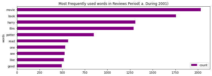
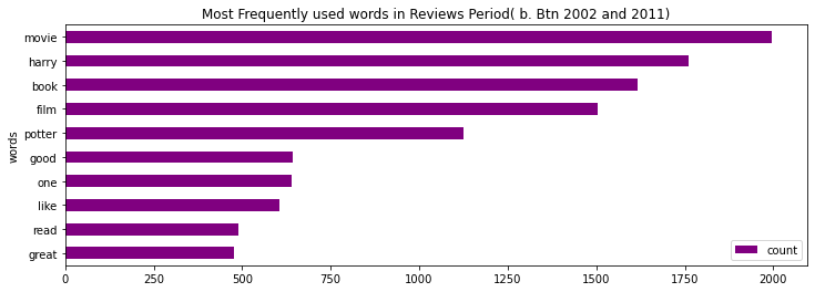
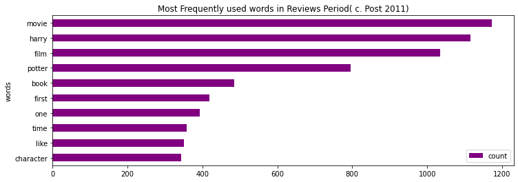
We can see that most of the words like “movie”, “harry”, “film”, and several other words are commonly written in the reviews.
However, we can get a better perspective if we look at 2 words. This is where n-grams come into play. The above analysis is uni-gram or 1-gram, i.e. we analyzed the frequency of each word. Similarly, we can look at bi-gram, where we analyze the frequency of 2 consecutive words. Also, we can look at tri-gram, where we analyze the frequency of 3 consecutive words. Let us understand n-gram computation using an example.
e.g. Sentence = “Text Analysis is an important part in NLP.”
Here, unigrams = {“Text”, “Analysis”, “is”, “an”, “important”, “part”, “in”, “NLP”}
bi-grams = { “Text Analysis”, “Analysis is”, “is an”, “an important”, “important part”, “part in”, “in NLP” }
tri-grams = { “Text Analysis is”, “Analysis is an” , “is an important” , “an important part”, “important part in” , “part in NLP” }
7. EDA: Looking at the top bi-grams mentioned in the reviews
counts_no = collections.Counter(ngrams(token_list, 2))
clean_reviews = pd.DataFrame(counts_no.most_common(30), columns=['words', 'count'])
fig, ax = plt.subplots(figsize=(12, 8))
clean_reviews.sort_values(by='count').plot.barh(x='words', y='count', ax=ax, color="purple")
ax.set_title("Most Frequently used Bigrams in Reviews")
plt.show()
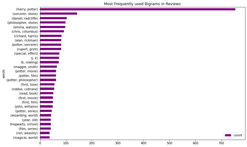
Insight:
- The most bi-grams are “harry potter”, followed by “sorcerer stone” and so on.
- If we analyze closely, we can look at the top 30 bi-grams also contain names of actors – “daniel radcliffe”, “emma watson”, “alan rickman” and others.
- Also, the director’s name “chris columbus” appears in the top bi-grams.
- There is also mention of “film series”. It means that there can be prequels or sequels to this movie. Let us note it and see what unfolds in the next analysis.
- There is also mention of the “wizarding world” and “magical world”. This gives an indication that the movie is about wizards and magic.
- This is pretty awesome. So far, no spoilers.
Let’s look at the top 10 bi-grams for each of the time periods.
for period in sorted(df['Period'].unique()):
    lemmatized_tokens = list(df[df['Period']==period]['review_lemmas'])
    token_list = list(itertools.chain(*lemmatized_tokens))
    counts_no = collections.Counter(ngrams(token_list, 3))
    clean_reviews = pd.DataFrame(counts_no.most_common(10), columns=['words', 'count'])
    fig, ax = plt.subplots(figsize=(12, 4))
    clean_reviews.sort_values(by='count').plot.barh(x='words', y='count', ax=ax, color="purple")
    ax.set_title("Most Frequently used bi-grams in Reviews Period( "+str(period)+")")
    plt.show()
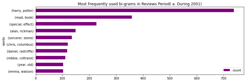
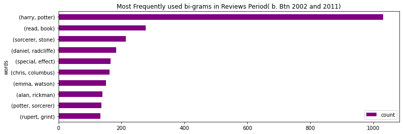

Some excellent insights are visible.
- The bi-gram “harry potter” is on the top for all 3 periods. Similarly, “chris columbus” consistently ranks the 6th most important bi-gram.
- “alan rickman” (the actor who played Snape) ranked 4th in Period 1, and its rank decreased to 8 in Period 2 and finally decreased to a rank of 10 by Period 3. This indicates that “alan rickman” is losing popularity among the reviewers.
- Similarly, “daniel radcliffe” (the actor who played harry potter) ranked 7th in Period 1, and its rank improved to 4 in Period 2 and finally to a rank of 3 by Period 3. This indicates that “daniel radcliffe” is gaining popularity among the reviewers.
8. EDA: Looking at the top tri-grams mentioned in the reviews
counts_no = collections.Counter(ngrams(token_list, 3))
clean_reviews = pd.DataFrame(counts_no.most_common(30), columns=['words', 'count'])
fig, ax = plt.subplots(figsize=(12, 8))
clean_reviews.sort_values(by='count').plot.barh(x='words', y='count', ax=ax, color="purple")
ax.set_title("Most Frequently used Trigrams in Reviews")
plt.show()
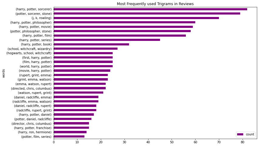
We see tri-grams like “j k rowling”, “hogwarts school witchcraft”. We can understand that it is about some witchcraft school. Again, exciting as we learn new information.
Let’s look at the top 10 tri-grams for each time period.
for period in sorted(df['Period'].unique()):
    lemmatized_tokens = list(df[df['Period']==period]['review_lemmas'])
    token_list = list(itertools.chain(*lemmatized_tokens))
    counts_no = collections.Counter(ngrams(token_list, 3))
    clean_reviews = pd.DataFrame(counts_no.most_common(10), columns=['words', 'count'])
    fig, ax = plt.subplots(figsize=(12, 4))
    clean_reviews.sort_values(by='count').plot.barh(x='words', y='count', ax=ax, color="purple")
    ax.set_title("Most Frequently used tri-grams in Reviews Period( "+str(period)+")")
    plt.show()


Nothing insightful here.
9. EDA: Wordclouds
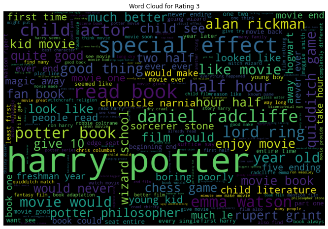
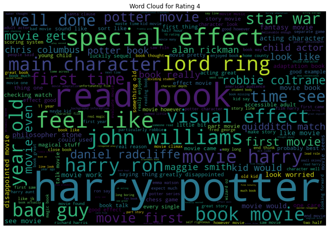
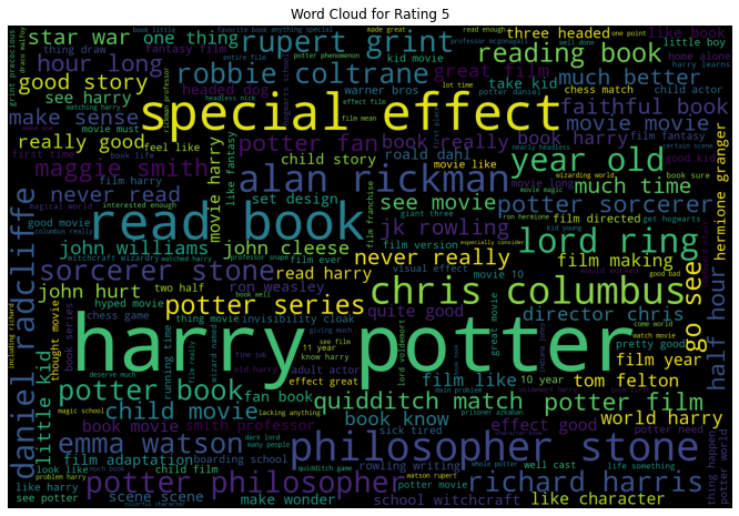
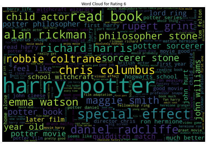
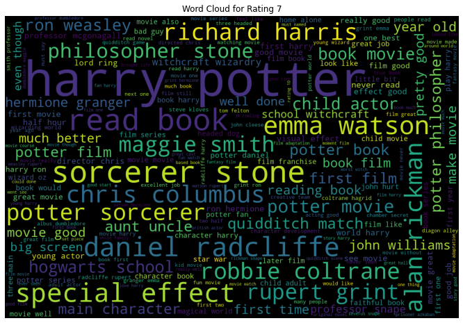
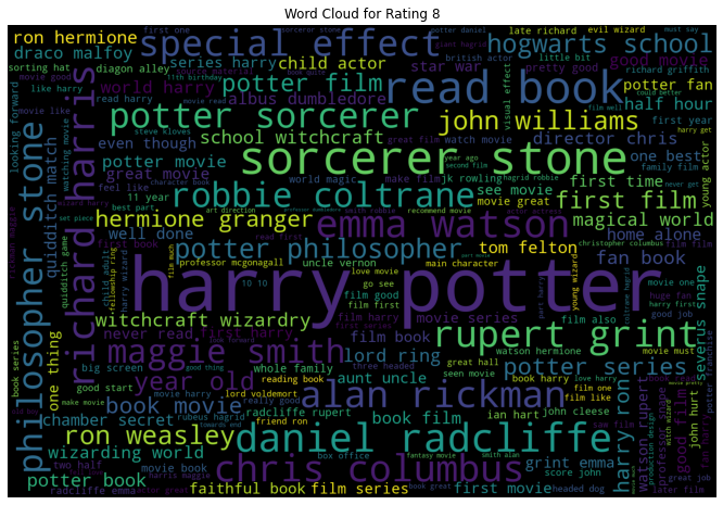
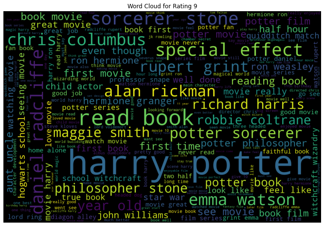
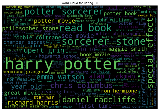
We saw in the above EDA that the bi-grams convey much information for our review data. In that sense, let us look at the word cloud created using bi-grams for each rating individually. A word cloud is a visual that helps to understand the most frequent words appearing in the text corpus.
for rating in range(1,11):
    curr_lemmatized_tokens = list(df[df['Rating']==rating]['review_lemmas'])
    vectorizer = CountVectorizer(ngram_range=(2,2))
    bag_of_words = vectorizer.fit_transform(df[df['Rating']==rating]['review_lemmas'].apply(lambda x : ' '.join(x)))
    sum_words = bag_of_words.sum(axis=0)
    words_freq = [(word, sum_words[0, idx]) for word, idx in vectorizer.vocabulary_.items()]
    words_freq =sorted(words_freq, key = lambda x: x[1], reverse=True)
    words_dict = dict(words_freq)
    WC_height = 1000
    WC_width = 1500
    WC_max_words = 200
    wordCloud = WordCloud(max_words=WC_max_words, height=WC_height, width=WC_width)
    wordCloud.generate_from_frequencies(words_dict)
    plt.figure(figsize=(20,8))
    plt.imshow(wordCloud)
    plt.title('Word Cloud for Rating '+str(rating))
    plt.axis("off")
    plt.show()
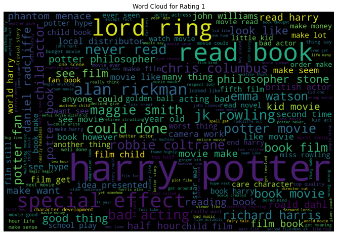
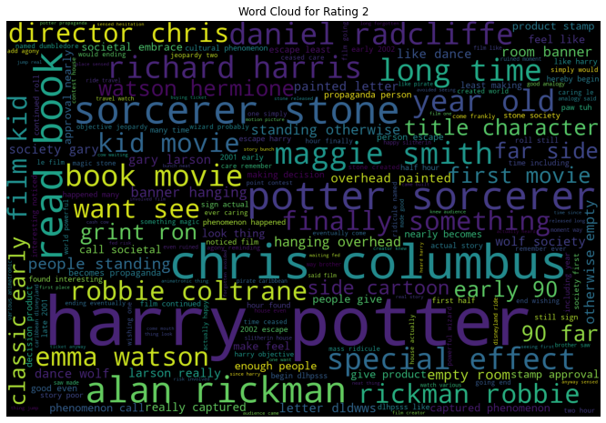
Insights:
- When Rating is 1, we see bi-grams like “bad acting”, “see hype”, etc. Also, we can see mention of “phantom menace” and “lord rings”. It appears that reviewers are comparing the Harry potter movie with movies like “Star Wars: Phantom Menace” and “Lord of the rings”.
- When the Rating is 2, we see bi-grams like “otherwise empty”, “standing otherwise”, etc.
- When Rating is 3, we see bi-grams like “quidditch game”, “chess game”, etc.
- When Rating is 4, we see bi-grams like “main character”, “bad guy”, etc.
- When the Rating is 5, we see bi-grams like “reading book”, “really good”, etc.
- When the Rating is 6, we see bi-grams like “school witchcraft”, “quidditch match”, etc.
- When Rating is 7, we see bi-grams like “child actor”, “big screen”, etc.
- When Rating is 8, we see bi-grams like “book movie”, “wizarding world”, etc.
- When Rating is 9, we see bi-grams like “great job”, “well done”, etc.
- When the Rating is 10, we see bi-grams like “10 10”, “love movie”, etc. Also, we can see mention of “chamber secret”. This is the 2nd movie of the Harry Potter series.
All the word clouds did have the names of the movie, the characters, and the actors portraying those characters.
So, after all this exercise, we have learned that the movie is
- Based on a book.
- It has special effects comparable to “Star Wars: Phantom Menace” and “Lord of the rings”.
- Has child actors.
- It is about magic and wizarding school.
- Has a chess and quidditch game.
Again, after all the analysis, we have not faced any spoilers but have got a good gist of the movie plot.
Conclusion
This article analysed the IMDB reviews of the movie “Harry Potter and the Sorcerer’s Stone” using NLP. We started by understanding the data, then did some EDA and performed necessary text processing and NLP. The movie was released in 2001, so we analysed:
- The change in ratings over the last 20 years.
- The popularity trend of the actors or characters portraying those actors.
- Frequent words, bi-grams, and tri-grams occurred within the reviews.
- The change in review size (i.e., total words in review) over time
- The reviews’ writing style and Interpretation (simple or complicated to read) over time.
Key takeaways
- Text analysis using NLP is compelling and can give some interesting insights.
- The entire exercise can be applied to any other movie or series, and you could use NLP. You can use any other corpus and apply a similar text analysis.
Thanks for reading my article on NLP! I hope you like it. Share in the comments below. If you wish to read more articles on NLP, head to our blog.
Feel free to connect with me on LinkedIn if you want to discuss this with me.
The media shown in this article is not owned by Analytics Vidhya and is used at the Author’s discretion.


