Introduction
A lead in a business, also known as a sales lead, is a user or a potential customer who has shown interest in what your company has to offer. Leads are generally captured by tracking the user’s actions, like how much they visit the website, asking them to fill up some forms, etc.
Leads are then used by the people in the company’s sales and marketing team to target the audience with a higher chance of converting into a sale. For the sales and marketing team to be efficient, the leads should be scored so that they can be easily sorted from higher probability to lower probability of conversion. This whole process is called lead scoring.
Now, let’s talk about Exploratory Data Analysis (EDA). It is an integral part of any Machine Learning and Data Science project, as while performing EDA, one can learn about the data and make inferences/insights from it. No machine learning model is complete without a proper EDA done over it, as it helps in feature extraction & deletion and decides the best algorithm to develop the model.
In this article, we will only perform Exploratory Data Analysis over a Lead Scoring Dataset, which will help you understand how to move forward with such a dataset, as lead scoring is a widespread practice in product or service-based companies.
What is Exploratory Data Analysis?
Exploratory Data Analysis or EDA is an important part of any Data Science or Data Analysis project. The philosophy behind EDA is to examine and learn about the data before building any model. It investigates the dataset to discover anomalies (outliers), patterns, and relations and forms hypotheses based on understanding the given dataset. It is generally classified into two methods, i.e., graphical analysis and non-graphical analysis.
The following things are part of EDA:
- Get maximum insights from the dataset
- Uncover underlying structure
- Extract important features from the dataset
- Detect outliers and anomalies(if any)
- Test assumptions
EDA is essential because it is a good practice to understand the problem statement and the various relationships between the data features before getting your hands dirty.
Why is EDA important for an ML project?
EDA makes understanding the dataset’s structure easy, making data modelling easier. The primary goal of EDA is to make data ‘clean’, implying that it should be devoid of anomalies, outliers, and redundancies. It helps identify the incorrect data points so they may be readily removed from the dataset.
Technically, the primary motive of EDA is to:
- Examine the data distribution
- Handling missing values and outliers
- Removing duplicate data
- Encoding the categorical variables
- Normalizing and Scaling
It gives you a clear picture of the features and their relationships. Providing guidelines for essential features, removing non-essential features, and ensuring the correctness and effectiveness of data used.
Case study On Exploratory Data Analysis
Problem Statement:
We need to perform EDA over the given Lead Scoring dataset and make out as many as possible inferences.
Explaining Dataset:
The dataset can be found on this link.
The original dataset contains a total of 37 columns and 9240 rows. But to keep this article short and informative, we will consider only the most important columns/features, which I extracted after performing EDA on the original data. If you want, you can also work on the original dataset!
Description of all the columns considered for this article:
| Variables | Description |
| Prospect ID | A unique ID with which the customer is identified. |
| Lead Origin | The origin identifier with which the customer was identified to be a lead. Includes API, Landing Page Submission, etc. |
| Lead Source | The source of the lead. Includes Google, Organic Search, Olark Chat, etc. |
| Converted | The target variable. Indicates whether a lead has been successfully converted or not. |
| Time Spent on Website | The total time spent by the customer on the website. |
| Last Activity | Last activity performed by the customer. Includes Email Opened, Olark Chat Conversation, etc. |
| Specialization | The industry domain in which the customer worked before. Includes the level ‘Select Specialization’, meaning the customer had not selected this option while filling out the form. |
| What is your current occupation | Indicates whether the customer is a student, unemployed or employed. |
| City | The city of the customer. |
You can find the original Data Dictionary here.
Data Preparation:
Now, we can start with the practical implementation.
As the dataset is big, we won’t be investing a lot of time in data preparation. We will focus more on EDA part i.e., making insights.
Now we will import all the required libraries and the dataset.
# Supress warnings
import warnings
warnings.filterwarnings("ignore")

# Importing Libraries
import numpy as np
import pandas as pd
import matplotlib.pyplot as plt
import seaborn as sns
# Visualization
from matplotlib.pyplot import xticks
%matplotlib inline
# Data display customization
pd.set_option('display.max_rows', 20)
pd.set_option('display.max_columns', 100)
pd.options.display.max_rows = 100
# Loading Dataset
data = pd.read_csv('Leads.csv')
# List of all the columns, to be dropped from the original data:
drop_list = ['How did you hear about X Education',

             'Lead Profile','Asymmetrique Activity Index',

             'Asymmetrique Activity Score',

             'Asymmetrique Profile Index',

             'Asymmetrique Profile Score',

             'Lead Number',

             'What matters most to you in choosing a course',

             'Search',

             'Magazine',

             'Newspaper Article',

             'X Education Forums',

             'Newspaper',

             'Digital Advertisement',

             'Through Recommendations',

             'Receive More Updates About Our Courses',

             'Update me on Supply Chain Content',

             'Get updates on DM Content',

             'I agree to pay the amount through cheque',

             'A free copy of Mastering The Interview',
             'Country']

# Dropping the columns

data = data.drop(drop_list, axis=1)

print(data.head())
Checking whether the dataset has duplicated values or not:
sum(data.duplicated(subset = 'Prospect ID')) == 0
The output of the above code is True; hence, there are no duplicate rows in the dataset.
NOTE: There are a lot of ‘Select’ values for many columns, as the customer did not select any option from the given list while filling out the form. These ‘Select’ values are as good as NULL, so we must replace them with NaN.
data = data.replace('Select', np.nan)
Let’s check how many null values are there in the dataset:
data.isna().sum()
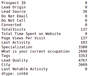
We will be replacing NaN values in the int64/float64 data type columns with the mean of the column and the in the object type columns with the mode of the column. You can deal with null values much better, but for this article, we are following the simplest way to deal with them.
for col in data.columns:
    if data[col].dtypes == 'int64' or data[col].dtypes == 'float64':
        data[col].fillna(data[col].mean(), inplace=True)
    else:
        data[col].fillna(data[col].mode()[0], inplace=True)
So, now we are done with data preparation, we can start EDA.
Exploratory Data Analysis (EDA):
1. Converted
# Converted is the target variable, Indicating whether a lead has been successfully converted (1) or not (0).
data['Converted'].value_counts()

# here we check, how much converison has happened
converted = round(sum(data['Converted']) / len(data['Converted'])*100, 2)
print(converted,'%')
# Output: 38.54 %
2. Lead Origin
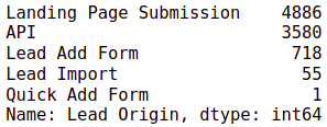
# we check the value counts in Lead Origin
data['Lead Origin'].value_counts()
# we drop the value with 1 occurence
data.drop(data.index[data['Lead Origin'] == 'Quick Add Form'], inplace=True)
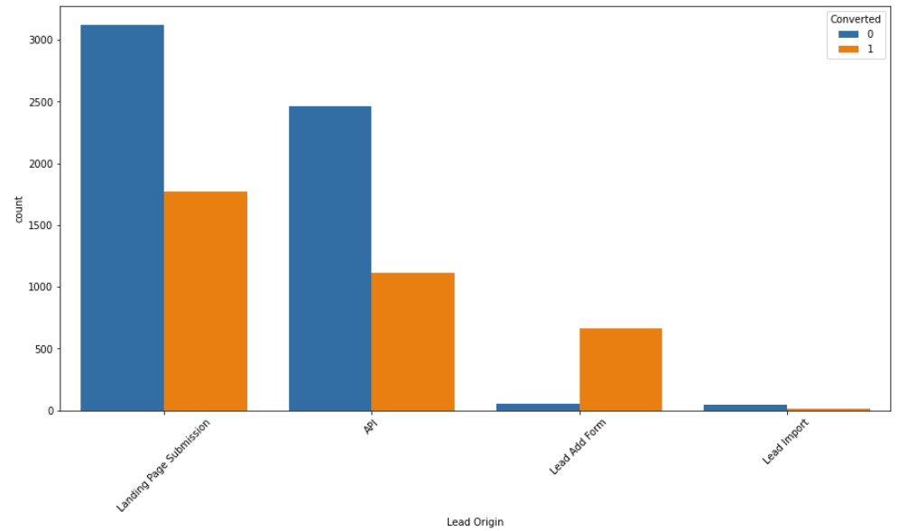
# we plot the value counts with respect to the target variable
fig, axs = plt.subplots(figsize = (15,7.5))
sns.countplot(x = "Lead Origin", hue = "Converted", data = data, order = data['Lead Origin'].value_counts().index)
xticks(rotation = 45)
plt.show()
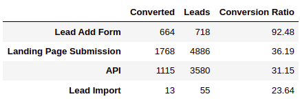
# here we calculate the conversion ratio for each value in Lead Origin
d = {}
for val in data['Lead Origin'].unique():
    a = data[data['Lead Origin'] == val]['Converted'].sum()
    b = data[data['Lead Origin']==val]['Converted'].count()
    d[val] = [a, b, round(a/b*100, 2)]
pd.DataFrame.from_dict(d, orient='index').rename(columns = {0: 'Converted', 1: 'Leads',2: 'Conversion Ratio'}).sort_values(by=['Conversion Ratio'], ascending=False)
INFERENCE:
- The maximum number of leads originated from “Landing Page Submission”, but the conversion % was low i.e. 36.19%.
- “Lead Add Form” was the best performing Lead Origin with 92.48% conversion %.
3. Lead Source
data['Lead Source'].value_counts()
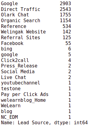
# there are 5 "google", we can replace it with "Google"
# we can see there are a lot of values with very less occurences
# we can replace all of then with "Others"

data['Lead Source'] = data['Lead Source'].replace(['google'], 'Google')
data['Lead Source'] = data['Lead Source'].replace(['Click2call',
'Live Chat',
                                                   'NC_EDM',
                                                   'Pay per Click Ads',
                                                   'Press_Release',
                                                   'Social Media',
                                                   'WeLearn',
                                                   'bing',
                                                   'blog',
                                                   'testone',
                                                   'welearnblog_Home',
                                                   'youtubechannel'], 'Others')
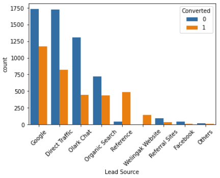
# plotting count plot w.r.t target variable
sns.countplot(x = "Lead Source", hue = "Converted", data = data, order = data['Lead Source'].value_counts().index)
xticks(rotation = 45)
plt.show()
# conversion ratio
d = {}
for val in data['Lead Source'].unique():
    a = data[data['Lead Source'] == val]['Converted'].sum()
    b = data[data['Lead Source']==val]['Converted'].count()
    d[val] = [a, b, round(a/b*100, 2)]
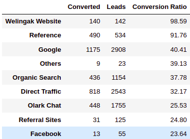
pd.DataFrame.from_dict(d, orient='index').rename(columns = {0: 'Converted', 1: 'Leads',2: 'Conversion Ratio'}).sort_values(by=['Conversion Ratio'], ascending=False)
INFERENCE:
- The Source with the maximum number of leads is “Google” & “Direct Traffic,” but it has less conversion.
- “Welingak Website” and “Reference” were the best performing Lead Sources with 98.59% and 91.76% conversions, respectively.
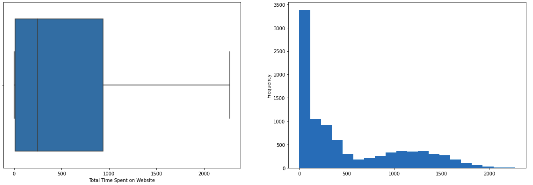
4. Total Time Spent on Website
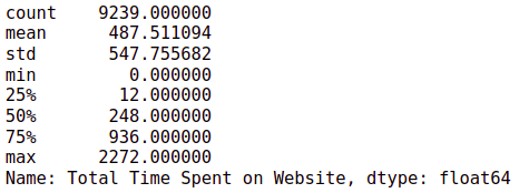
data['Total Time Spent on Website'].describe()
# plotting boxplot and histogram
fig, axs = plt.subplots(1,2,figsize = (20,6.5))
sns.boxplot(data['Total Time Spent on Website'], ax = axs[0])
data['Total Time Spent on Website'].plot.hist(bins=20, ax = axs[1])
plt.show()
# plotting boxplot w.r.t. the target variable
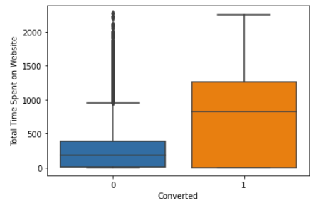
sns.boxplot(y = 'Total Time Spent on Website', x = 'Converted', data = data)
plt.show()
INFERENCE:
- There are no outliers in the data.
- The column is Right Skewed.
- Leads with more time spent on the website are more likely to be converted.
5. Last Activity
data['Last Activity'].value_counts()
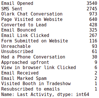
# Let's keep considerable last activities as such and club all others to "Other_Activity"
data['Last Activity'] = data['Last Activity'].replace(['Had a Phone Conversation',
                                                       'View in browser link Clicked',
                                                       'Visited Booth in Tradeshow',
                                                       'Approached upfront',
                                                       'Resubscribed to emails',
                                                       'Email Received',
                                                       'Email Marked Spam'], 'Other_Activity')
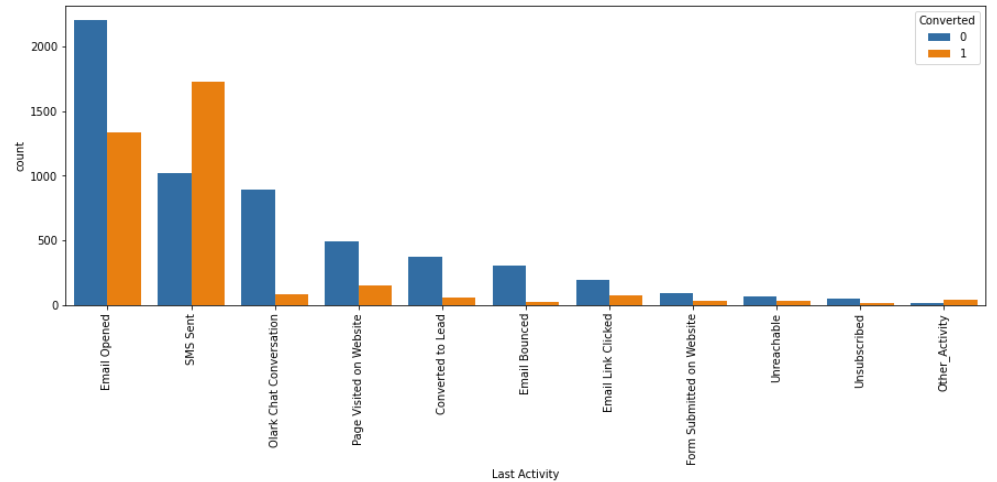
# plotting the counplot w.r.t. the target variable
fig, axs = plt.subplots(figsize = (15,5))
sns.countplot(x = "Last Activity", hue = "Converted", data = data, order = data['Last Activity'].value_counts().index)
xticks(rotation = 90)
plt.show()
# conversion ratio
d = {}
for val in data['Last Activity'].unique():
    a = data[data['Last Activity'] == val]['Converted'].sum()
    b = data[data['Last Activity']==val]['Converted'].count()
    d[val] = [a, b, round(a/b*100, 2)]
pd.DataFrame.from_dict(d, orient='index').rename(columns = {0: 'Converted', 1: 'Leads',2: 'Conversion Ratio'}).sort_values(by=['Conversion Ratio'], ascending=False)
INFERENCE:
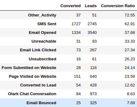
- “Email Opened” and “SMS Sent” were the last activities that generated the maximum number of leads and were also good in conversion ratio.
- “SMS Sent” was the best performing Last Activity with a 62.91% conversion ratio.
6. Specialization
data['Specialization'].value_counts()
# plotting the countplot w.r.t. the target variable
fig, axs = plt.subplots(figsize = (15,5))

sns.countplot(x = "Specialization", hue = "Converted", data = data, order = data['Specialization'].value_counts().index)

xticks(rotation = 90)

plt.show()
# conversion ratio
d = {}
for val in data['Specialization'].unique():
    a = data[data['Specialization'] == val]['Converted'].sum()
    b = data[data['Specialization']==val]['Converted'].count()
    d[val] = [a, b, round(a/b*100, 2)]
pd.DataFrame.from_dict(d, orient='index').rename(columns = {0: 'Converted', 1: 'Leads',2: 'Conversion Ratio'}).sort_values(by=['Conversion Ratio'], ascending=False)
INFERENCE:
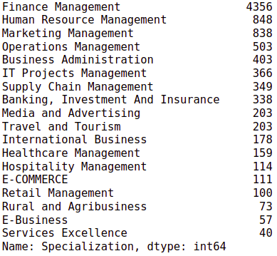
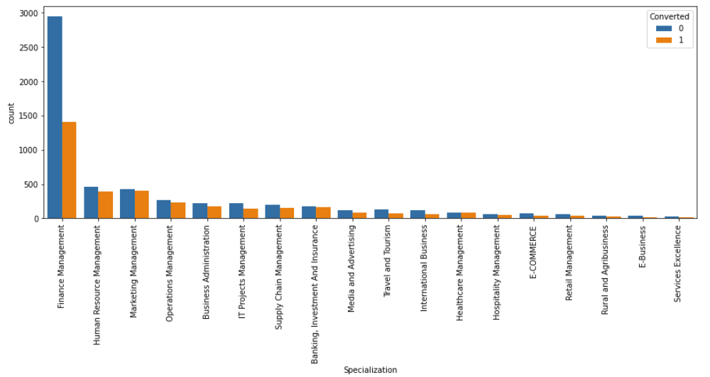
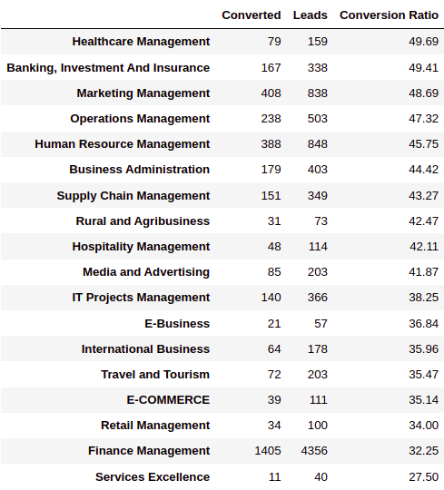
- “Finance Management” generated the maximum number of leads, but the conversion ratio was just 32.25%.
- “Healthcare Management” was the best performing Specialization with a 49.69% conversion ratio.
7. What is your current occupation
data['What is your current occupation'].value_counts()

# plotting the countplot w.r.t. the target variable
fig, axs = plt.subplots(figsize = (15,5))
sns.countplot(x = "What is your current occupation", hue = "Converted", data = data, order = data['What is your current occupation'].value_counts().index)
xticks(rotation = 90)
plt.show()
# converison ratio
d = {}
for val in data['What is your current occupation'].unique():
    a = data[data['What is your current occupation'] == val]['Converted'].sum()
    b = data[data['What is your current occupation']==val]['Converted'].count()
    d[val] = [a, b, round(a/b*100, 2)]
pd.DataFrame.from_dict(d, orient='index').rename(columns = {0: 'Converted', 1: 'Leads',2: 'Conversion Ratio'}).sort_values(by=['Conversion Ratio'], ascending=False)
INFERENCE:
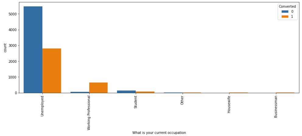
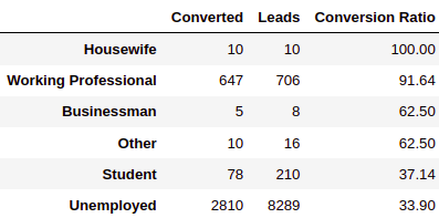
- The “Unemployed” occupation generated the maximum number of leads but had the least conversion ratio.
- The “Working Professional” occupation was the best performing Occupation with a 91.64% conversion ratio, “Housewife” occupation had a 100% conversion ratio, but we are not considering it due to fewer data points.
8. City
data['City'].value_counts()
# plotting the countplot w.r.t. the target variable
fig, axs = plt.subplots(figsize = (15,5))
sns.countplot(x = "City", hue = "Converted", data = data, order = data['City'].value_counts().index)
xticks(rotation = 90)
plt.show()
# conversion ratio
d = {}
for val in data['City'].unique():
    a = data[data['City'] == val]['Converted'].sum()
    b = data[data['City']==val]['Converted'].count()
    d[val] = [a, b, round(a/b*100, 2)]
pd.DataFrame.from_dict(d, orient='index').rename(columns = {0: 'Converted', 1: 'Leads',2: 'Conversion Ratio'}).sort_values(by=['Conversion Ratio'], ascending=False)
INFERENCE:
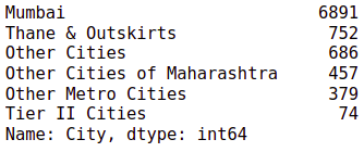
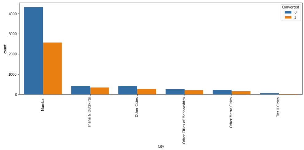
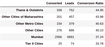
- “Mumbai” generated the maximum number of leads, but the conversion ratio was just 32.24%.
- All cities have almost the same conversion ratio, b/w 33% to 44%.
Conclusion
In this article, we understood the meaning of Exploratory Data Analysis (EDA) and why it is essential in ML projects with the help of a case study. We looked at how we could analyze the dataset and draw inferences from the same. Some of the key takeaways from the articles are:
- Understanding what leads are, how they are useful to a company, what lead scoring is, and EDA & why EDA is done before any ML project.
- Understanding a Lead Scoring dataset from kaggle, containing 37 columns and 9240 rows. The dataset is from an education company, containing data about the leads generated by the potential buyers for the company’s services or products. We have to use the given data to perform EDA over it and make inferences. To keep this article short, we are only using 8 features.
- Dealing with null values present in object type columns and int/float type columns, both have a different approach to dealing with missing values.
- Performing graphical and non-graphical EDA over the dataset, we used a count and box plot for graphical EDA. For non-graphical EDA, we used value counts, ratios, etc., to make inferences.
- Making out inferences using EDA like, finding out the best performing value from each column, finding out which value generated most and least leads, finding out relations between columns, etc.


%202.jpg)