Implementing Count Vectorizer and TF-IDF in NLP using PySpark

Introduction

Natural language processing is one of the most widely used skills at the enterprise level as it can deal with non-numeric data. As we know machines communicate in either 0 or 1. Still, we as humans communicate in our native languages (English as a second language in most regions), so we need a technique from which we can iterate through our language and make the machine understand that. For that NLP helped us with a wide range of tools, this is the second article discussing tools used in NLP using PySpark.

In this article, we will move forward to discuss two tools of NLP that are equally important for natural language processing applications, and they are:

1. TF-IDF: TF-IDF is abbreviated as the Term frequency-inverse document frequency, which is designed to get how much the words are relevant in the corpus.
2. Count Vectorizer: The main aim of Count Vectorizer is to convert the string document into Vectorize token.

So let’s deep dive into the rest of the two NLP tools so that in the next article, we can build real-world NLP applications using PySpark.

This article was published as a part of the Data Science Blogathon.

Start the Spark Session

Before implementing the above-mentioned tools we first need to start and initiate the Spark Session to maintain the distributed processing, for the same, we will be importing the SparkSession module from PySpark.

from pyspark.sql import SparkSession

spark_nlp2 = SparkSession.builder.appName('nlp_tools_2').getOrCreate()
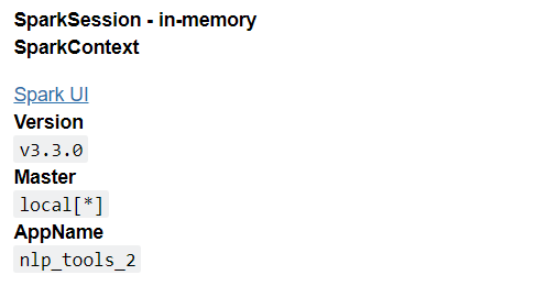
spark_nlp2

Output:

Inference: The hierarchy of functions is used to create the PySpark Session where the builder function will build the environment where Pyspark can fit in then appName will give the name to the session and get or create() will eventually create the Spark Session with a certain configuration.

TF-IDF in NLP

TF-IDF is one of the most decorated feature extractors and stimulators tools where it works for the tokenized sentences only i.e., it doesn’t work upon the raw sentence but only with tokens; hence first, we need to apply the tokenization technique (it could be either basic Tokenizer of RegexTokenizer as well depending on the business requirements). Now when we have the token so we can implement this algorithm on top of that, and it will return the importance of each token in that document. Note that it is a feature vectorization method, so any output will be in the format of vectors only.

Now, let’s breakdown the TF-IDF method; it is a two-step process:

Term Frequency (TF)

As the name suggests, term frequency looks for the total frequency for the particular word we wanted to consider to get the relation in the whole document corpus. There are several ways to execute the Term Frequency step.

• Count: This is a raw count that will return the number of times a word/token occurred in a document.
• Count/Total number of words: This will return the term frequency after dividing the total count of occurrence of words by the total number of words in the corpus.
• Boolean frequency: It has the most basic method to consider whether the term occurred or not i.e., if the term occurred, then the value will be 1; otherwise 0.
• Logarithmically scaled: Frequency is counted based on the formulae (log(1 + raw count)).

Inverse Document Frequency

While the term frequency looks for the occurrence of a particular word in the document corpus at the other end, IDF has a pretty subjective and critical job to execute, where it kind of classifies words based on how common and uncommon they are among the whole document.

from pyspark.ml.feature import HashingTF, IDF, Tokenizer

sentenceData = spark_nlp2.createDataFrame([
    (0.0, "Hi I heard about Spark"),
    (0.0, "I wish Java could use case classes"),
    (1.0, "Logistic regression models are neat")
], ["label", "sentence"])

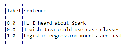
sentenceData.show(truncate=False)

Output

Code Breakdown

1. The very first step is to import the required libraries to implement the TF-IDF algorithm for that we imported HashingTf (Term frequency), IDF(Inverse document frequency), and Tokenizer (for creating tokens).
2. Next, we created a simple data frame using the createDataFrame() function and passed in the index (labels) and sentences in it.
3. Now we can easily show the above dataset using Pyspark’s show function, keeping the truncate parameter as False so that the whole sentence is visible.

tokenizer = Tokenizer(inputCol="sentence", outputCol="words")
wordsData = tokenizer.transform(sentenceData)
wordsData.show(truncate=False)

Output

Code Breakdown

1. As we discussed above, we first need to go through the Tokenization process for working with TF-IDF. Hence, the Tokenizer object is created to break down sentences into tokens.
2. After creating the instance of the tokenizer object, we need to transform it so that changes are visible. Then in the last step, we showed the “words” column, where the sentence is broken down into tokens.

hashingTF = HashingTF(inputCol="words", outputCol="rawFeatures", numFeatures=20)
featurizedData = hashingTF.transform(wordsData)

idf = IDF(inputCol="rawFeatures", outputCol="features")
idfModel = idf.fit(featurizedData)
rescaledData = idfModel.transform(featurizedData)

rescaledData.select("label", "features").show(truncate=False)

Output

Code Breakdown

In this part, we are implementing the TF-IDF as we are all done with the pre-requisite required to execute it.

1. The process starts by creating the HashingTf object for the term frequency step where we pass the input, output column, and a total number of features and then transform the same to make the changes in the data frame.
2. Now comes the part of executing the IDF process. First, we are creating the IDF object and only passing the input and output columns.
3. Now we are fitting the IDF model, and one can notice that for that, we are first using the fit function and then the transform method on top of featured data (just like the K-Means algorithm).

Conclusion of TF-IDF

In the output, we can see that from a total of 20 features, it first indicates the occurrence of those related features ([6,8,13,16]) and then shows us how much they are common to each other.

CountVectorizer in NLP

Whenever we talk about CountVectorizer, CountVectorizeModel comes hand in hand with using this algorithm. A trained model is used to vectorize the text documents into the count of tokens from the raw corpus document. Count Vectorizer in the backend act as an estimator that plucks in the vocabulary and for generating the model. Note that this particular concept is for the discrete probability models.

Enough of the theoretical part now. Let’s do our hands dirty in implementing the same.

rom pyspark.ml.feature import CountVectorizer

df = spark_nlp2.createDataFrame([
    (0, "a b c".split(" ")),
    (1, "a b b c a".split(" "))
], ["id", "words"])

# fit a CountVectorizerModel from the corpus.
cv = CountVectorizer(inputCol="words", outputCol="features", vocabSize=3, minDF=2.0)

model = cv.fit(df)

result = model.transform(df)
result.show(truncate=False)

Output

Code Breakdown

1. Firstly we started with importing the CountVectorizer from the ml. feature library.
2. Then we will create the dummy data frame from the createDataFrame function. Note that each row we are creating here is a bag of words with specific IDs.
3. Now, as the last step, we will fit and transform the CountVectorizerModel from the corpus by passing the vocab size as 3 so that the features are evaluated on the same basis.
4. Looking at the output, we can see that vocalizing and mind emphasizing 3 words from the vocab are taken into account.

Conclusion

Here we are in the last section of the article, where we will discuss everything we did regarding the TF-IDF algorithm and CountVectorizerModel in this article. Firstly we gathered the theoretical knowledge about each algorithm and then did the practical implementation of the same.

1. First, we started with some background information regarding the NLP tools that we have already covered and what new things we will now cover.
2. Then we move to TF-IDF model/algorithm and discussed it in depth by breaking it down, and after acquiring the theoretical knowledge, we implemented the same and got the desired results.
3. Similarly, we did the same for CountVectorizerModel, i.e., learning about how it works and why we use it and then implementing the same to get the results.

Here’s the repo link to this article. I hope you liked my article on Guide for implementing Count Vectorizer and TF-IDF in NLP using PySpark. If you have any opinions or questions, comment below.

Connect with me on LinkedIn for further discussion on MLIB or otherwise.

Frequently Asked Questions

The media shown in this article is not owned by Analytics Vidhya and is used at the Author’s discretion.

Aman Preet