This article was published as a part of the Data Science Blogathon.
Introduction
Standardization is one of the feature scaling techniques which scales down the data in such a way that the algorithms (like KNN, Logistic Regression, etc.) which are dependent on distance and weights should not get affected by uneven-scaled datasets because if it happens, then, the model accuracy will not be good (will show this practically), on the other hand, if we will scale the data evenly in such a way that the data points are mean centric and standard deviation of the distribution is 1 then the weights will be treated equally by the algorithm giving the more relevant and accurate results.
In this article, we will not only see how we can do standard scaling in machine learning using Python, but also the effects of scaling. Comparison between the distribution (before and after scaling) so that one can understand how scaling is affecting the sample space and, last but not least, the effect on outliers which will show us whether standard scaling helps in removing the outliers or not.
import numpy as np # linear algebra
import pandas as pd # data processing
import matplotlib.pyplot as plt
import seaborn as sns
We are importing some required libraries, which will help in practically implementing standardization.
- Numpy: For solving equations related to linear algebra.
- Pandas: For DataFrame manipulation and preprocessing.
- Matplotlib and Seaborn: For data visualization and seeing the distributions.
import numpy as np # linear algebra
import pandas as pd # data processing
# import matplotlib.pyplot as plt
# import seaborn as sns

df = pd.read_csv('Social_Network_Ads.csv')
df=df.iloc[:,2:]
print(df.sample(5))
df = pd.read_csv('Social_Network_Ads.csv')
df=df.iloc[:,2:]
df.sample(5)
Hit Run to see the output
Inference: For practically implementing the standardization technique we are using the Social Networking Advertisement Agency dataset. Note that here I’m keeping only needful columns so that the focus should be on the concept rather than understanding the complexity of the dataset. Explore the dataset by looking at a different set of samples.
Train Test Split
from sklearn.model_selection import train_test_split
X_train, X_test, y_train, y_test = train_test_split(df.drop('Purchased', axis=1),
                                                    df['Purchased'],
                                                    test_size=0.3,
                                                    random_state=0)

X_train.shape, X_test.shape
Output:
((280, 2), (120, 2))
Inference: There will always be a debate about whether to do a train test split before doing standard scaling or not, but in my preference, it is essential to do this step before standardization as if we scale the whole data, then for our algorithm, there might be no testing data left which will eventually lead to overfitting condition. On the other hand now if we only scale our training data then we will still have the testing data which is unseen for the model.
Standard Scaler
from sklearn.preprocessing import StandardScaler

scaler = StandardScaler()

# fit the scaler to the train set, it will learn the parameters
scaler.fit(X_train)

# transform train and test sets
X_train_scaled = scaler.transform(X_train)
X_test_scaled = scaler.transform(X_test)
Code breakdown:
- Before applying the standard scaling, we need to import the StandardScaler module from SKLEARN.preprocessing and initiate the instance of that object.
- Then we are using the fit function only to train the training dataset. This is important, as we discussed, to avoid the condition of overfitting, we only use a training dataset.
- The third step, to imply standard scaling is to transform the training and testing dataset. Note that here we are using the entire dataset not only the training dataset.
scaler.mean_
Output:
array([3.78642857e+01, 6.98071429e+04])
Inference: Above output is all about the corresponding mean values that we got for both features after doing the mean centric during the standardization process.
X_train_scaled = pd.DataFrame(X_train_scaled, columns=X_train.columns)
X_test_scaled = pd.DataFrame(X_test_scaled, columns=X_test.columns)
Inference: Though we had X_train and X_test in the form of DataFrame still when we will see the X_train_scaled and X_test_scaled then, it will return the NumPy array structure for that we are first converting it into DataFrame.
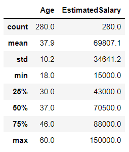
np.round(X_train.describe(), 1)
Output:
np.round(X_train_scaled.describe(), 1)
Output:
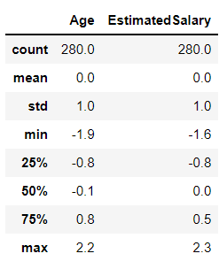
Inference: The above two output is just for keeping a note of the mean value for both cases (Scaled and Pre-Scaled data). Where Pre-Scaled dataset has some mean value and standard deviation, while on the other hand Scaled data have 0 mean and 1 standard deviation, and if this condition pertains then that means we have successfully scaled the dataset.
Effect of Scaling
In this section of the article, we will see the possible effects of standardization on the model’s accuracy and on what type of algorithms these techniques are useful. Let’s just jump in and do some visualization.
fig, (ax1, ax2) = plt.subplots(ncols=2, figsize=(12, 5))

ax1.scatter(X_train['Age'], X_train['EstimatedSalary'])
ax1.set_title("Before Scaling")
ax2.scatter(X_train_scaled['Age'], X_train_scaled['EstimatedSalary'],color='red')
ax2.set_title("After Scaling")
plt.show()
Output:
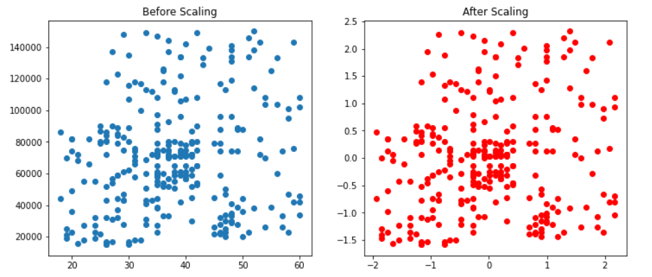
Inference: Don’t go for red and blue dots in the above plot because they will be the same. The real difference is in the X and Y scale; after scaling, we can see that the mean has shifted in such a way that now it is in origin (the condition of standard scaling).
fig, (ax1, ax2) = plt.subplots(ncols=2, figsize=(12, 5))

# before scaling
ax1.set_title('Before Scaling')
sns.kdeplot(X_train['Age'], ax=ax1)
sns.kdeplot(X_train['EstimatedSalary'], ax=ax1)

# after scaling
ax2.set_title('After Standard Scaling')
sns.kdeplot(X_train_scaled['Age'], ax=ax2)
sns.kdeplot(X_train_scaled['EstimatedSalary'], ax=ax2)
plt.show()
Output:
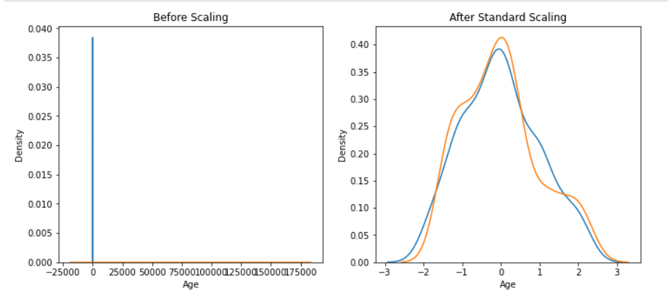
Inference: Now look at the probability density function using the KDE plot for both scaled and non-scaled data. In the case of non-scaled data, we can only see the Age on the Y-axis and the Estimated salary on the X-Axis this is because the data is not evenly scaled, but on the other side, when the scaling is done then, both the features are flowing well across the sample space.
Comparison of Distributions
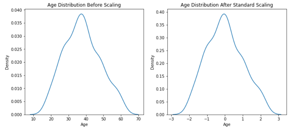
Here we will compare the distribution plot for Age and Estimated Salary distribution and find out whether after the process of standardization will there be any effect on the distribution of the dataset or not.
fig, (ax1, ax2) = plt.subplots(ncols=2, figsize=(12, 5))

# before scaling
ax1.set_title('Age Distribution Before Scaling')
sns.kdeplot(X_train['Age'], ax=ax1)

# after scaling
ax2.set_title('Age Distribution After Standard Scaling')
sns.kdeplot(X_train_scaled['Age'], ax=ax2)
plt.show()
Output:
fig, (ax1, ax2) = plt.subplots(ncols=2, figsize=(12, 5))

# before scaling
ax1.set_title('Salary Distribution Before Scaling')
sns.kdeplot(X_train['EstimatedSalary'], ax=ax1)

# after scaling
ax2.set_title('Salary Distribution Standard Scaling')
sns.kdeplot(X_train_scaled['EstimatedSalary'], ax=ax2)
plt.show()
Output:
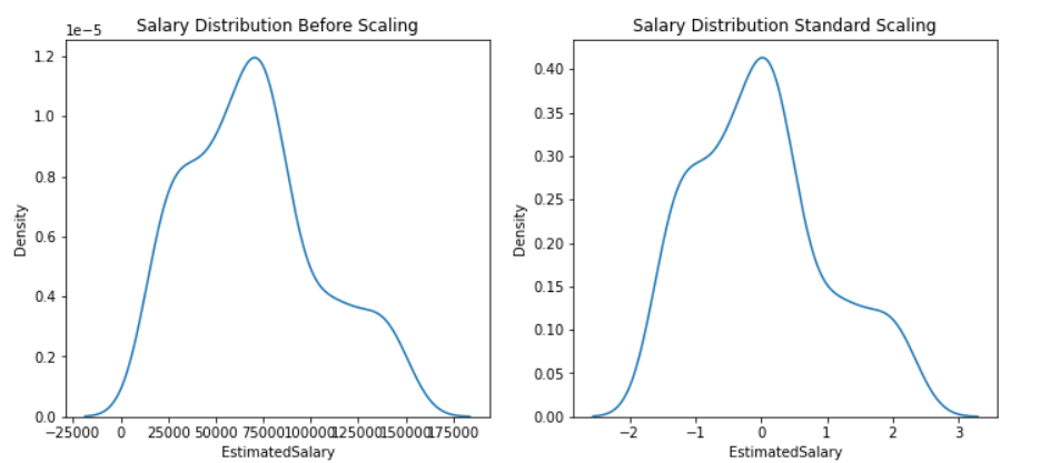
Inference: In the above two plots we have seen both the features in both situations i.e. before scaling, and after scaling and got conclusive evidence that standardization doesn’t change the distribution it will be the same just the scale of the data will be changed.
Why is Scaling Important?
By far, we saw how scaling can affect the distribution and nature of the dataset. Now it’s time to see why scaling is important before model building or how it can improve the model’s accuracy. Along with that, we will also see what type of algorithm shows the effect for that, we have taken two algorithms, i.e., Logistic regression, where there is a lot of significance of distance, and another one is Decision Tree which has no relationship with distance.
So, let’s find out how both algorithms will react to standard scaling.
from sklearn.linear_model import LogisticRegression

# Building Logistic Regression instance
lr = LogisticRegression()
lr_scaled = LogisticRegression()

# Model training
lr.fit(X_train,y_train)
lr_scaled.fit(X_train_scaled,y_train)

# Storing the predictions of both scaled and pre-scaled data
y_pred = lr.predict(X_test)
y_pred_scaled = lr_scaled.predict(X_test_scaled)

from sklearn.metrics import accuracy_score
print("Actual",accuracy_score(y_test,y_pred))
print("Scaled",accuracy_score(y_test,y_pred_scaled))
Output:
Actual 0.6583333333333333
Scaled 0.8666666666666667
Inference: In the above code, we imported Logistic Regression first and followed every step the same as we did before to scale the data using a standard scaler, and when we compared the accuracy of the model of Actual data with the Scaled data then we found out that scaling the data in the case of this algorithm helps quite well as the accuracy increased from 65% to 87%.
from sklearn.tree import DecisionTreeClassifier

dt = DecisionTreeClassifier()
dt_scaled = DecisionTreeClassifier()

dt.fit(X_train,y_train)
dt_scaled.fit(X_train_scaled,y_train)

y_pred = dt.predict(X_test)
y_pred_scaled = dt_scaled.predict(X_test_scaled)

print("Actual",accuracy_score(y_test,y_pred))
print("Scaled",accuracy_score(y_test,y_pred_scaled))
Output:
Actual 0.875
Scaled 0.875
Inference: As we did in the case of the previous ML algorithm same, we did in the case of the Decision Tree classifier but in this case, we can see that scaling has not improved the accuracy of the model as scaling is helpful in the algorithms like KNN, PCA and other which are dependent on distance.
Effect of Outlier After Standardization
This is the last thing that we will discuss in the course of this article, where we will learn about the effect of outliers after standardization, i.e., if standard scaling can remove the outliers or it has no effect on them. So let’s quickly find that out.
df = df.append(pd.DataFrame({'Age':[5,90,95],'EstimatedSalary':[1000,250000,350000],'Purchased':[0,1,1]}),ignore_index=True)
df
Output:
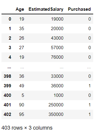
Inference: In the above code, we are appending (adding) three new data points, and by the values of those data points, we can assume that they will be outliers in the entire sample space.
plt.scatter(df['Age'], df['EstimatedSalary'])
Output:
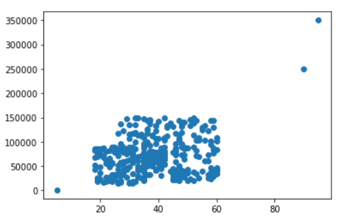
Inference: In the above plot we can see three altogether different data points, which are surely an outlier that we just imputed in the original dataset.
from sklearn.model_selection import train_test_split
X_train, X_test, y_train, y_test = train_test_split(df.drop('Purchased', axis=1),
                                                    df['Purchased'],
                                                    test_size=0.3,
                                                    random_state=0)

X_train.shape, X_test.shape
Output:
((282, 2), (121, 2))
As mentioned in the beginning about the Train test split, it is a good practice to follow this technique before using standard scaling (recommended but not necessary).
from sklearn.preprocessing import StandardScaler

scaler = StandardScaler()

# fit the scaler to the train set, it will learn the parameters
scaler.fit(X_train)

# transform train and test sets
X_train_scaled = scaler.transform(X_train)
X_test_scaled = scaler.transform(X_test)
Inference: Again, following the same process for standardizing the dataset using StandardScaler‘s fit function on the training set and transforming both the testing and training set.
X_train_scaled = pd.DataFrame(X_train_scaled, columns=X_train.columns)
X_test_scaled = pd.DataFrame(X_test_scaled, columns=X_test.columns)
fig, (ax1, ax2) = plt.subplots(ncols=2, figsize=(12, 5))

ax1.scatter(X_train['Age'], X_train['EstimatedSalary'])
ax1.set_title("Before Scaling")
ax2.scatter(X_train_scaled['Age'], X_train_scaled['EstimatedSalary'],color='red')
ax2.set_title("After Scaling")
plt.show()
Output:
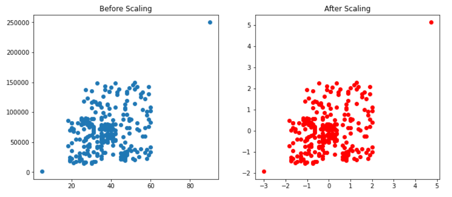
Inference: From the above code, we have plotted both stimulations before and after scaling and from the results, it is visible that standard scaling does not affect outliers, as the data points have not changed their positions at all.
Conclusion
This is the last section of the article, where we will try to cover everything we discussed so far in this article but a nutshell so that this segment will act like a revision and concepts refresher, so let’s just get started.
- First, we got started with the introduction part, where we discussed standard scaling and then we came to know the importance of train test split before applying standardization.
- Then we compared the distribution of the dataset in both cases, i.e., for actual and after scaling datasets to which, after looking at the distribution, we got conclusive evidence that distributions are not changed.
- Then we learned about why scaling is important by comparing the two most used algorithms (but with different mathematics intuition behind them). The last topic was the effect on outliers, to which we saw the plot and inference that there is no effect of outliers.
The media shown in this article is not owned by Analytics Vidhya and is used at the Author’s discretion.


