Learning Time Series Analysis & Modern Statistical Models

Introduction

Statistical models are significant for understanding and predicting complex data. You can see patterns and relationships and make accurate predictions about future values. A viable area for statistical modeling is time-series analysis.

Time series data are collected over time and can be found in various fields such as finance, economics, and technology. Statistical models can be used to better understand this kind of data, generate meaningful insights, and make predictions that help make critical decisions. These models are mathematical representations of data behavior and can be used to predict future values. From simple autoregressive models to more complex integrated moving average models, this model offers a variety of options for analyzing and forecasting time series data.

This article reviews various statistical models commonly used in time-series analysis, their strengths and weaknesses, and how to implement them in real-world applications. Before discussing them, everyone should know what time-series analysis is.

Learning Objectives

1. Understand what are moving average values.
2. Learn how to implement this model using several python libraries.
3. Familiarity with various statistical models used for time-series analysis.
4. Understand the advantages and disadvantages of Time-Series Analysis.

This article was published as a part of the Data Science Blogathon.

Table of Content

1. What is Time-Series Analysis?
2. Fundamentals of Auto-regressive Models
3. Understanding Moving Average Models
4. Autoregressive Integrated Moving Average Models: An Overview
5. Vector autoregression
6. Hierarchical time series models: An Introduction
7. Exploring Variations in Statistical Models for Time Series
8. Advantages and Disadvantages of using Statistical Methods for Time Series
9. Conclusion

What is Time-Series Analysis?

Time-series analysis is the study of data points collected over time. It’s about identifying patterns, trends, and relationships in your data. It aims to predict future values based on past data and is a powerful tool for gaining meaningful insights and predictions from data collected over time.

Time-series analysis looks at continuously collected data points, such as daily stock prices or monthly sales figures. Analyzing this data allows you to identify patterns, trends, and relationships that help predict future value. The statistical model is one of the essential tools in time-series analysis. These models are mathematical representations of time series behavior and can be used to predict future values. There are various types of statistical models developed for time-series analysis.

The autoregressive model, Moving average model, Autoregressive model with an integrated moving average model, Vector autoregression model, Variation in statistical models, and hierarchical time series model each have their strengths and weaknesses, and choosing the suitable model depends on the characteristics of the time series and the purpose of your analysis.

Source – Databrio.com

Fundamentals of Auto-regressive Models

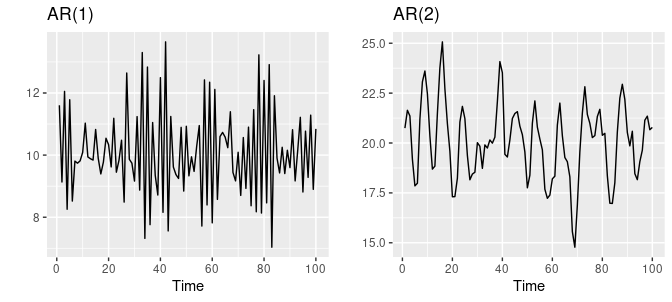
Autoregressive (AR) models are popular and influential time-series analysis and forecasting tools. It assumes that the underlying process generating the data is a linear combination of past observations. This model describes a time series as a linear combination of past values commonly used to predict future trends. It is based on the idea that the current value of a time series is dependent on previous values.

AR models are beneficial for modeling univariate time series data, aiming to predict future values based on past observations. The model’s order (p) is defined by the number of past observations used to estimate the current value. The model is trained on historical data, and the coefficients are determined by minimizing the difference between the predicted and actual values. The model can then forecast future values of the time series data.

Source – otexts.com

The main advantage of AR models is the ability to understand time series dynamics by calculating past values. This is especially useful for time series showing trends and patterns.

However, AR models have some limitations. One of the limitations is the assumption of linearity between current and past values. This is not always the case. Also, a large amount of data is required to make accurate predictions.

Here is the code, which shows how we work with AR models in Python. I recommend you do it in R since it is widely used for statistical analysis, but here I used Python since everyone is familiar with it.

from statsmodels.tsa.ar_model import AR
import numpy as np
#generate data
data = np.random.randn(100)
#fit model
model = AR(data)
model_fit = model.fit()
#make prediction
yhat = model_fit.predict(len(data), len(data))
print(yhat)

Understanding Moving Average Models

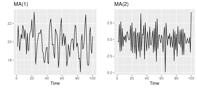
A moving average (MA) model is a statistical model commonly used in time-series analysis. This model is based on the idea that past mistakes influence the future value of a time series in the forecast. Unlike autoregressive (AR) models, which use past values to make predictions, moving average models use historical errors or residuals.

The model is trained on historical data, and the coefficients are determined by minimizing the difference between the predicted and actual values. The model can then forecast future values of the time series data.

It helps identify and assess the impact of irregular or unexpected events. In moving average models, the current value of a time series is modeled as a linear combination of past errors or residuals. The order of the model (q) is defined by the number of past errors used to predict the current error term.

It is also worth noting that MA models are often combined with Auto-Regressive (AR) models to create a more powerful forecasting tool called ARIMA (Auto-Regressive Integrated Moving Average).

Source – otexts.com

One of the main advantages of MA models is the ability to understand the impact of unexpected events and errors over time.

Identify and assess the effect of irregular or random events. However, there are some restrictions: linearity assumptions and the need for large amounts of data.

Here is the simple Python code.

from statsmodels.tsa.arima_model import ARMA
import numpy as np
#generate data
data = np.random.randn(100)
#fit model
model = ARMA(data, order=(0, 1))
model_fit = model.fit()
#make prediction
yhat = model_fit.predict(len(data), len(data))
print(yhat)

Autoregressive Integrated Moving Average Models: An Overview

The autoregressive integrated moving average model is a statistical model commonly used in time-series analysis. ARIMA models are a popular method for analyzing and forecasting time series data. They are beneficial for modeling time series data that exhibit patterns such as seasonality, trend, and noise.

The ARIMA model combines three components: autoregression, integration, and moving average. The autoregression component models the dependence between an observation and a number of lag observations. This component is used to model the persistence of time series data.

The integration component models the dependence between an observation and the differences between consecutive observations. This component is used to model the trend of time series data. The moving average component models the dependence between an observation and a residual error from a moving average model. These component models random fluctuations or noise in time series data.

ARIMA models are a powerful tool for analyzing time series data and can provide valuable insights into the underlying structure of the data.

The main advantage of ARIMA models is their ability to capture trends and seasonal ingredients in time series. It helps deal with non-stationary time series and can be used with standard statistical techniques to improve forecast accuracy.

Although, it has limitations, such as linearity assumptions and a large amount of data required.

Here is the simple Python code for how we use the ARIMA model.

from statsmodels.tsa.arima_model import ARIMA
import numpy as np
#generate data
data = np.random.randn(100)
#fit model
model = ARIMA(data, order=(1, 1, 1))
model_fit = model.fit()
#make prediction
yhat = model_fit.predict(len(data), len(data))
print(yhat)

Vector Autoregression

Vector autoregression (VAR) is a statistical model to explore and analyze dynamic relationships between multiple periods. It extends the autoregressive (AR) model and can simultaneously model various dependent variables. In contrast, VAR models the dependence between multiple variables and their lag values.

In VAR models, each variable is modeled as a linear combination of the past values of all variables and a random error term. The model is estimated using the least squares method, and the parameters are typically estimated using maximum likelihood estimation. VAR models can include exogenous variables, also called explanatory variables, because the variables are not modeled as autoregressive variables.

The model had this variable as an additional term in the equation. Matrix multiplication is used to represent linear relationships between variables in VAR models. The model’s coefficients are represented as a matrix, and the previous values of the variable are multiplied by this matrix to get the predicted values. As the order of the model increases, so does the complexity of the model, allowing for more accurate predictions.

One of the main advantages of VAR models is their ability to capture dynamic correlations between multiple time series. It helps you understand how changes in one variable affect other variables and can also be used to predict various variables simultaneously.

Nevertheless, they have several limitations, such as being computationally expensive, assuming linearity, and requiring large amounts of data.

Hierarchical Time Series Models: An Introduction

A hierarchical time series model is a statistical model used to analyze and forecast time series data arranged in a hierarchical structure. A hierarchical structure refers to a data set with multiple levels of aggregation.

These are divided into various levels in a hierarchical time series model, such as region, department, and development. A separate time series model was then fitted to each dataset. These model parameters are combined to create predictions for the entire data set.

Source – stackoverflow.com

One of the main advantages of hierarchical time series models is their ability to handle complex data structures and account for differences between groups. It also helps detect and predict changes in trends and patterns at various hierarchical levels. This is widely used in business and economics, such as retail sales forecasting, budgeting, and other planning activities.

When the number of levels or the number of units at each level is increased, they can become more complex and computationally expensive.

Exploring Variations in Statistical Models for Time Series

Several variations on statistical models can be used for analyzing and forecasting time series data, but I have listed some of the most important ones. They are

Exponential Smoothing Models: These models are used for forecasting time series data that exhibit trends and/or seasonality. They are based on weighting recent observations more heavily than older ones.

State Space Models: These models are used for modeling dynamic systems with unobserved variables. They are particularly useful for modeling time series data with complex patterns.

GARCH Models: These models are used for modeling time series data with volatility that changes over time. They are commonly used in finance for modeling stock returns and other financial time series data.

Structural Time Series Models: This model is used for modeling time series with an underlying structure and a stochastic component. They are used to model the underlying causal factors of a time series.

Machine Learning Models: These models are used for forecasting time series data using techniques such as neural networks, decision trees, and support vector machines. They are particularly useful for modeling time series data with complex patterns and non-linear relationships.

Advantages of using Statistical Methods for Time-Series Analysis

Explanation: Many statistical methods are based on simple mathematical formulas and are easy to understand and explain. This makes it easier for others to interpret the results and use them to make decisions.

Robustness: Statistical methods can be designed to be robust to outliers and other forms of noise in the data, which can be critical in many applications. Efficiency: Many statistical methods are computationally efficient, making it possible to analyze large and complex time series data sets.

Reliability: Statistical methods are generally more reliable with outliers and other data types and are suitable for use with real-world data.

Forecasting: Statistical methods can be used to make forecasts of future values of the time series. This can be useful for decision-making, budgeting, and other planning activities.

Completeness: Statistical methods have been developed and used for many years, and a wealth of knowledge and software is available to make our job easy. While statistical methods for time-series analysis have many advantages, there are also some potential disadvantages to consider

While statistical methods for time-series analysis have many advantages, there are also some potential disadvantages to consider

Disadvantages of using Statistical Methods for Time-Series Analysis

Assumptions: Many statistical methods make assumptions about critical data properties such as stationarity, linearity, and normality that cannot be met in practice.

Complexity: Some statistical methods, such as VAR and SSM, are very complex and require a high degree of expertise to apply and interpret them.

Data requirements: Some statistical methods require a large amount of data to produce accurate results, which can be problematic if the data is limited or of poor quality.

Data Quality: Statistical methods rely on high-quality data, and poor-quality data can lead to inaccurate results.

Overfitting: Some models may fit the data too well and may not generalize well to new data.

Limited Accuracy: Statistical methods rely on past observations and cannot capture future events not included in past data.

Conclusion

Statistical methods are a powerful tool for analyzing and forecasting time series data. They can provide valuable insights into the underlying structure of the data and make predictions about future values. There are various types of statistical models available, each with its strengths and weaknesses, that can be used for different types of time series data.

However, it’s important to be aware of the assumptions and requirements of the chosen model. In addition, it’s essential to carefully consider the characteristics of the time series data before applying any statistical method. Additionally, it is important to note that statistical methods are not the only approach to time-series analysis. It’s always worthwhile to consider other methods and models as well.

Furthermore, it’s important to remember that the results obtained using statistical methods should always be critically evaluated. Domain knowledge should be used to interpret and make sense of the results.

Key Takeaways

• Time-series analysis is a powerful tool for understanding and forecasting patterns and trends in data over time.
• Statistical methods, such as Autoregressive (AR), Moving Average (MA), Autoregressive Integrated Moving Average (ARIMA), Vector Autoregression (VAR), and Hierarchical time series models, etc. are widely used to analyze time series data.
• Each of these methods has its advantages and disadvantages. The choice of method depends on the specific characteristics of the time series data and the research question being addressed.
• It’s critical to remember that no single model is suitable for all time series data. Therefore, a combination of models and techniques may be necessary for accurate predictions.
• It’s key to thoroughly understand the underlying assumptions and limitations of the models to ensure accurate predictions and conclusions.
• These models can be implemented using various Python, R, and other programming language libraries.
• In summary, statistical methods for time-series analysis provide a flexible and powerful tool for understanding and forecasting time-series data.
• However, it’s critical to be aware of their limitations and to use them in conjunction with other methods and domain knowledge.

Want to share something not mentioned above? Thoughts? Feel free to comment below.

The media shown in this article is not owned by Analytics Vidhya and is used at the Author’s discretion.

Gayathri

I am Gayathri studying masters in data science. I am always curious to learn new things in this emerging world. The data science field makes me more fascinated and interested.I love reading books and doing projects.