Top 100 Data Science Interview Questions and Answers 2025

Imagine stepping into your first data science interview—your palms are sweaty, your mind racing, and then… you get a question you actually know the answer to. That’s the power of preparation. With data science reshaping how businesses make decisions, the race to hire skilled data scientists is more intense than ever. For freshers, standing out in a sea of talent means more than just knowing the basics—it means being interview-ready. In this article, we’ve handpicked the top 100 data science interview questions that frequently appear in real interviews, giving you the edge you need.

From Python programming and EDA to statistics and machine learning, each question is paired with insights and tips to help you master the concepts and ace your answers. Whether you’re aiming for a startup or a Fortune 500 company, this guide is your secret weapon to land that dream job and kickstart your journey as a successful data scientist.

Data Science Interview Questions Regarding Python

Let us look at data science interview questions and answers regarding Python.

Beginner Interview Python Questions for Data Science

Q1. Which is faster, python list or Numpy arrays, and why?

A. NumPy arrays are quicker than Python lists when it comes to numerical computations. NumPy is a Python library for array processing, and it offers several functions for performing operations on arrays in an efficient manner.

One of the reasons NumPy arrays are faster than Python lists is that NumPy arrays are written in C, whereas Python lists are written in Python. This implies that operations on NumPy arrays are written in a compiled language and hence are faster than operations on Python lists, which are written in an interpreted language.

Q2. What is the difference between a python list and a tuple?

A. A list in Python is a sequence of objects of varying kinds. Lists are mutable, i.e., you can alter the value of a list item or insert or delete items in a list. Lists are defined using square brackets and a comma-delimited list of values.

A tuple is also an ordered list of objects, but it is immutable, meaning that you cannot alter the value of a tuple object or add or delete elements from a tuple.

Lists are initiated using square brackets ([ ” ]), whereas tuples are initiated using parentheses ((”, )).

Lists have a number of built-in methods for adding, deleting, and manipulating elements, but tuples don’t have these methods.

Generally, tuples are quicker than lists in Python

Q3. What are python sets? Explain some of the properties of sets.

A. In Python, a set is an unordered collection of unique objects. Sets are often used to store a collection of distinct objects and to perform membership tests (i.e., to check if an object is in the set). Sets are defined using curly braces ({ and }) and a comma-separated list of values.

Here are some key properties of sets in Python:

• Sets are unordered: Sets do not have a specific order, so you cannot index or slice them like you can with lists or tuples.
• Sets are unique: Sets only allow unique objects, so if you try to add a duplicate object to a set, it will not be added.
• Sets are mutable: You can add or remove elements from a set using the add and remove methods.
• Sets are not indexed: Sets do not support indexing or slicing, so you cannot access individual elements of a set using an index.
• Sets are not hashable: Sets are mutable, so they cannot be used as keys in dictionaries or as elements in other sets. If you need to use a mutable object as a key or an element in a set, you can use a tuple or a frozen set (an immutable version of a set).

Q4. What is the difference between split and join?

A. Split and join are both functions of python strings, but they are completely different when it comes to functioning.

The split function is used to create a list from strings based on some delimiter, for eg. space.

a = ‘This is a string’
Li = a.split(‘ ‘)
print(li)

Output:

 [‘This’, ‘is’, ‘a’, ‘string’]

The join() method is a built-in function of Python’s str class that concatenates a list of strings into a single string. It is called on a delimiter string and invoked with a list of strings to be joined. The delimiter string is inserted between each string in the list when the strings are concatenated.

Here is an example of how to use the join() method:

 “ “.join(li)

Output:

This is a string

Here the list is joined with a space in between.

Q5. Explain the logical operations in python.

A. In Python, the logical operations and, or, and not can be used to perform boolean operations on truth values (True and False).

The and operator returns True if both the operands are True, and False otherwise.

The or operator returns True if either of the operands is True, and False if both operands are False.

The not operator inverts the boolean value of its operand. If the operand is True, not return False, and if the operand is False, not return True.

Q6. Explain the top 5 functions used for python strings.

A. Here are the top 5 Python string functions:

Function	Description
len()	Returns the length of a string.
strip()	Removes leading and trailing whitespace from a string.
split()	Splits a string into a list of substrings based on a delimiter.
replace()	Replaces all occurrences of a specified string with another string.
upper()	Converts a string to uppercase.
lower()	Converts a string to lowercase.

s = 'Hello, World!'

len(s)                  # 13
s.strip()               # 'Hello, World!'
s.split(',')            # ['Hello', ' World!']
s.replace('World', 'Universe')  # 'Hello, Universe!'
s.upper()               # 'HELLO, WORLD!'
s.lower()               # 'hello, world!'

Q7. What is the use of the pass keyword in python?

A. pass is a null statement that does nothing. It is often used as a placeholder where a statement is required syntactically, but no action needs to be taken. For example, if you want to define a function or a class but haven’t yet decided what it should do, you can use pass as a placeholder.

Q8. What is the use of the continue keyword in python?

A. continue is used in a loop to skip over the current iteration and move on to the next one. When continue is encountered, the current iteration of the loop is terminated, and the next one begins.

Intermediate Interview Python Data Science Questions

Q9. What are immutable and mutable data types?

A. In Python, an immutable object is an object whose state cannot be modified after it is created. This means that you can’t change the value of an immutable object once it is created. Examples of immutable objects in Python include numbers (such as integers, floats, and complex numbers), strings, and tuples.

On the other hand, a mutable object is an object whose state can be modified after it is created. This means that you can change the value of a mutable object after it is created. Examples of mutable objects in Python include lists and dictionaries.

Understanding the difference between immutable and mutable objects in Python is important because it can affect how you use and manipulate data in your code. For example, if you have a list of numbers and you want to sort the list in ascending order, you can use the built-in sort() method to do this. However, if you have a tuple of numbers, you can’t use the sort() method because tuples are immutable. Instead, you would have to create a new sorted tuple from the original tuple.

Q10. What is the use of try and accept block in python

A. The try and except block in Python are used to handle exceptions. An exception is an error that occurs during the execution of a program.

The try block contains code that might cause an exception to be raised. The except block contains code that is executed if an exception is raised during the execution of the try block.

Using a try-except block will save the code from an error to occur and can be executed with a message or output we want in the except block.

Q11. What are 2 mutable and 2 immutable data types in python?

A. 2 mutable data types are:

• Dictionary
• List

You can change/edit the values in a python dictionary and a list. It is not necessary to make a new list which means that it satisfies the property of mutability.

2 immutable data types are:

• Tuples
• String

You cannot edit a string or a value in a tuple once it is created. You need to either assign the values to the tuple or make a new tuple.

Q12. What are python functions, and how do they help in code optimization?

A.  In Python, a function is a block of code that can be called by other parts of your program. Functions are useful because they allow you to reuse code and divide your code into logical blocks that can be tested and maintained separately.

To call a function in Python, you simply use the function name followed by a pair of parentheses and any necessary arguments. The function may or may not return a value that depends on the usage of the turn statement.

Functions can also help in code optimization:

• Code reuse: Functions allow you to reuse code by encapsulating it in a single place and calling it multiple times from different parts of your program. This can help to reduce redundancy and make your code more concise and easier to maintain.
• Improved readability: By dividing your code into logical blocks, functions can make your code more readable and easier to understand. This can make it easier to identify bugs and make changes to your code.
• Easier testing: Functions allow you to test individual blocks of code separately, which can make it easier to find and fix bugs.
• Improved performance: Functions can also help to improve the performance of your code by allowing you to use optimized code libraries or by allowing the Python interpreter to optimize the code more effectively.

Q13. Why does NumPy have huge popularity in the field of data science?

A. NumPy (short for Numerical Python) is a popular library for scientific computing in Python. It has gained a lot of popularity in the data science community because it provides fast and efficient tools for working with large arrays and matrices of numerical data.

NumPy provides fast and efficient operations on arrays and matrices of numerical data. It uses optimized C and Fortran code behind the scenes to perform these operations, which makes them much faster than equivalent operations using Python’s built-in data structures. It provides fast and efficient tools for working with large arrays and matrices of numerical data.

NumPy provides a large number of functions for performing mathematical and statistical operations on arrays and matrices.

It allows you to work with large amounts of data efficiently. It provides tools for handling large datasets that would not fit in memory, such as functions for reading and writing data to disk and for loading only a portion of a dataset into memory at a time.

NumPy integrates well with other scientific computing libraries in Python, such as SciPy (Scientific Python) and pandas. This makes it easy to use NumPy with other libraries to perform more complex data science tasks.

Q14. Explain list comprehension and dict comprehension.

A. List comprehension and dict comprehension are both concise ways to create new lists or dictionaries from existing iterables.

List comprehension is a concise way to create a list. It consists of square brackets containing an expression followed by a for clause, then zero or more for or if clauses. The result is a new list that evaluates the expression in the context of the for and if clauses.

Dict comprehension is a concise way to create a dictionary. It consists of curly braces containing a key-value pair, followed by a for clause, then zero or more for or if clauses. A result is a new dictionary that evaluates the key-value pair in the context of the for and if clauses.

Q15. What are global and local variables in python?

A. In Python, a variable that is defined outside of any function or class is a global variable, while a variable that is defined inside a function or class is a local variable.

A global variable can be accessed from anywhere in the program, including inside functions and classes. However, a local variable can only be accessed within the function or class in which it is defined.

It is important to note that you can use the same name for a global variable and a local variable, but the local variable will take precedence over the global variable within the function or class in which it is defined. 

# This is a global variable
x = 10
def func():
  # This is a local variable
  x = 5
  print(x)my_function
func()
print(x)

Output:

This will print 5 and then 10

In the example above, the x variable inside the func() function is a local variable, so it takes precedence over the global variable x. Therefore, when x is printed inside the function, it prints 5; when it is printed outside the function, it prints 10.

Q16. What is an ordered dictionary?

A. An ordered dictionary, also known as an OrderedDict, is a subclass of the built-in Python dictionary class that maintains the order of elements in which they were added. In a regular dictionary, the order of elements is determined by the hash values of their keys, which can change over time as the dictionary grows and evolves. An ordered dictionary, on the other hand, uses a doubly linked list to remember the order of elements, so that the order of elements is preserved regardless of how the dictionary changes.

Q17. What is the difference between return and yield keywords?

A. Return is used to exit a function and return a value to the caller. When a return statement is encountered, the function terminates immediately, and the value of the expression following the return statement is returned to the caller.

yield, on the other hand, is used to define a generator function. A generator function is a special kind of function that produces a sequence of values one at a time, instead of returning a single value. When a yield statement is encountered, the generator function produces a value and suspends its execution, saving its state for later

Advanced Python Interview Questions

Q18. What are lambda functions in python, and why are they important?

A. In Python, a lambda function is a small anonymous function. You can use lambda functions when you don’t want to define a function using the def keyword.

Lambda functions are useful when you need a small function for a short period of time. They are often used in combination with higher-order functions, such as map(), filter(), and reduce().

Here’s an example of a lambda function in Python:

x = lambda a : a + 10
x(5)
15

In this example, the lambda function takes one argument (a) and adds 10 to it. The lambda function returns the result of this operation when it is called.

Lambda functions are important because they allow you to create small anonymous functions in a concise way. They are often used in functional programming, a programming paradigm that emphasizes using functions to solve problems.

Q19. What is the use of the ‘assert’ keyword in python?

A. In Python, the assert statement is used to test a condition. If the condition is True, then the program continues to execute. If the condition is False, then the program raises an AssertionError exception.

The assert statement is often used to check the internal consistency of a program. For example, you might use an assert statement to check that a list is sorted before performing a binary search on the list.

It’s important to note that the assert statement is used for debugging purposes and is not intended to be used as a way to handle runtime errors. In production code, you should use try and except blocks to handle exceptions that might be raised at runtime.

Q20. What are decorators in python?

A. In Python, decorators are a way to modify or extend the functionality of a function, method, or class without changing their source code. Decorators are typically implemented as functions that take another function as an argument and return a new function that has the desired behavior.

A decorator is a special function that starts with the @ symbol and is placed immediately before the function, method, or class it decorates. The @ symbol is used to indicate that the following function is a decorator.

Interview Questions Regarding EDA and Statistics

Let us look at data science interview questions and answers regarding EDA and Statistics.

Beginner Interview Questions on Statistics

Q21. How to perform univariate analysis for numerical and categorical variables?

A. Univariate analysis is a statistical technique used to analyze and describe the characteristics of a single variable. It is a useful tool for understanding the distribution, central tendency, and dispersion of a variable, as well as identifying patterns and relationships within the data. Here are the steps for performing univariate analysis for numerical and categorical variables:

For numerical variables:

• Calculate descriptive statistics such as the mean, median, mode, and standard deviation to summarize the distribution of the data.
• Visualize the distribution of the data using plots such as histograms, boxplots, or density plots.
• Check for outliers and anomalies in the data.
• Check for normality in the data using statistical tests or visualizations such as a Q-Q plot.

For categorical variables.

• Calculate the frequency or count of each category in the data.
• Calculate the percentage or proportion of each category in the data.
• Visualize the distribution of the data using plots such as bar plots or pie charts.
• Check for imbalances or abnormalities in the distribution of the data.

Note that the specific steps for performing univariate analysis may vary depending on the specific needs and goals of the analysis. It is important to carefully plan and execute the analysis in order to accurately and effectively describe and understand the data.

Q22. What are the different ways in which we can find outliers in the data?

A. Outliers are data points that are significantly different from the majority of the data. They can be caused by errors, anomalies, or unusual circumstances, and they can have a significant impact on statistical analyses and machine learning models. Therefore, it is important to identify and handle outliers appropriately in order to obtain accurate and reliable results.

Here are some common ways to find outliers in the data:

• Visual inspection: Outliers can often be identified by visually inspecting the data using plots such as histograms, scatterplots, or boxplots.
• Summary statistics: Outliers can sometimes be identified by calculating summary statistics such as the mean, median, or interquartile range, and comparing them to the data. For example, if the mean is significantly different from the median, it could indicate the presence of outliers.
• Z-score: The z-score of a data point is a measure of how many standard deviations it is from the mean. Data points with a z-score greater than a certain threshold (e.g., 3 or 4) can be considered outliers.

There are many other methods for detecting outliers in the data, and the appropriate method will depend on the specific characteristics and needs of the data. It is important to carefully evaluate and choose the most appropriate method for identifying outliers in order to obtain accurate and reliable results.

Q23. What are the different ways by which you can impute the missing values in the dataset?

A. There are several ways that you can impute null values (i.e., missing values) in a dataset:

• Drop rows: One option is to simply drop rows with null values from the dataset. This is a simple and fast method, but it can be problematic if a large number of rows are dropped, as it can significantly reduce the sample size and impact the statistical power of the analysis.
• Drop columns: Another option is to drop columns with null values from the dataset. This can be a good option if the number of null values is large compared to the number of non-null values, or if the column is not relevant to the analysis.
• Imputation with mean or median: One common method of imputation is to replace null values with the mean or median of the non-null values in the column. This can be a good option if the data are missing at random and the mean or median is a reasonable representation of the data.
• Imputation with mode: Another option is to replace null values with the mode (i.e., the most common value) of the non-null values in the column. This can be a good option for categorical data where the mode is a meaningful representation of the data.
• Imputation with a predictive model: Another method of imputation is to use a predictive model to estimate the missing values based on the other available data. This can be a more complex and time-consuming method, but it can be more accurate if the data are not missing at random and there is a strong relationship between the missing values and the other data.

Q24. What are Skewness in statistics and its types?

A. Skewness is a measure of the symmetry of a distribution. A distribution is symmetrical if it is shaped like a bell curve, with most of the data points concentrated around the mean. A distribution is skewed if it is not symmetrical, with more data points concentrated on one side of the mean than the other.

There are two types of skewness: positive skewness and negative skewness.

• Positive skewness: Positive skewness occurs when the distribution has a long tail on the right side, with the majority of the data points concentrated on the left side of the mean. Positive skewness indicates that there are a few extreme values on the right side of the distribution that is pulling the mean to the right.
• Negative skewness: Negative skewness occurs when the distribution has a long tail on the left side, with the majority of the data points concentrated on the right side of the mean. Negative skewness indicates that there are a few extreme values on the left side of the distribution that is pulling the mean to the left.

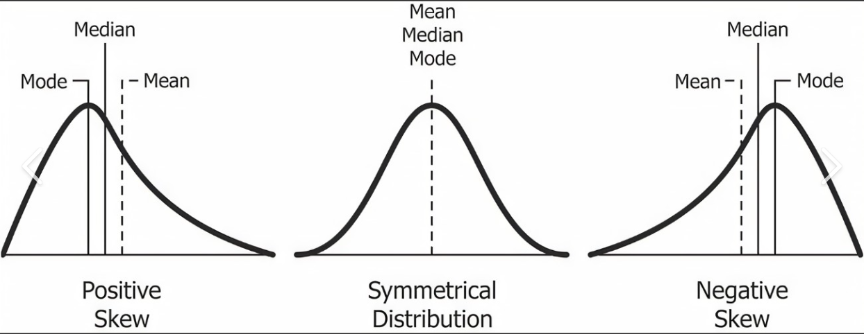
Q25. What are the measures of central tendency?

A. In statistics, measures of central tendency are values that represent the center of a dataset. There are three main measures of central tendency: mean, median, and mode.

The mean is the arithmetic average of a dataset and is calculated by adding all the values in the dataset and dividing by the number of values. The mean is sensitive to outliers, or values that are significantly higher or lower than the majority of the other values in the dataset.

The median is the middle value of a dataset when the values are arranged in order from smallest to largest. To find the median, you must first arrange the values in order and then locate the middle value. If there is an odd number of values, the median is the middle value. If there is an even number of values, the median is the mean of the two middle values. The median is not sensitive to outliers.

The mode is the value that occurs most frequently in a dataset. A dataset may have multiple modes or no modes at all. The mode is not sensitive to outliers.

Q26. Can you explain the difference between descriptive and inferential statistics?

A. Descriptive statistics is used to summarize and describe a dataset by using measures of central tendency (mean, median, mode) and measures of spread (standard deviation, variance, range). Inferential statistics is used to make inferences about a population based on a sample of data and using statistical models, hypothesis testing and estimation.

Q27. What are the key elements of an EDA report and how do they contribute to understanding a dataset?

A. The key elements of an EDA report include univariate analysis, bivariate analysis, missing data analysis, and basic data visualization. Univariate analysis helps in understanding the distribution of individual variables, bivariate analysis helps in understanding the relationship between variables, missing data analysis helps in understanding the quality of data, and data visualization provides a visual interpretation of the data.

Intermediate Interview Questions on Statistics for Data Science

Q28 What is the central limit theorem?

A. The Central Limit Theorem is a fundamental concept in statistics that states that as the sample size increases, the distribution of the sample mean will approach a normal distribution. This is true regardless of the underlying distribution of the population from which the sample is drawn. This means that even if the individual data points in a sample are not normally distributed, by taking the average of a large enough number of them, we can use normal distribution-based methods to make inferences about the population.

Q29. Mention the two kinds of target variables for predictive modeling.

A. The two kinds of target variables are:

Numerical/Continuous variables – Variables whose values lie within a range, could be any value in that range and the time of prediction; values are not bound to be from the same range too.

For example: Height of students – 5; 5.1; 6; 6.7; 7; 4.5; 5.11

Here the range of the values is (4,7)

And, the height of some new students can/cannot be any value from this range.

Categorical variable – Variables that can take on one of a limited, and usually fixed, number of possible values, assigning each individual or other unit of observation to a particular group on the basis of some qualitative property.

A categorical variable that can take on exactly two values is termed a binary variable or a dichotomous variable. Categorical variables with more than two possible values are called polytomous variables

For example Exam Result: Pass, Fail (Binary categorical variable)

The blood type of a person: A, B, O, AB (polytomous categorical variable)

Q30. What will be the case in which the Mean, Median, and Mode will be the same for the dataset?

A. The mean, median, and mode of a dataset will all be the same if and only if the dataset consists of a single value that occurs with 100% frequency.

For example, consider the following dataset: 3, 3, 3, 3, 3, 3. The mean of this dataset is 3, the median is 3, and the mode is 3. This is because the dataset consists of a single value (3) that occurs with 100% frequency.

On the other hand, if the dataset contains multiple values, the mean, median, and mode will generally be different. For example, consider the following dataset: 1, 2, 3, 4, 5. The mean of this dataset is 3, the median is 3, and the mode is 1. The dataset contains multiple values, and no value occurs with 100% frequency.

It is important to note that outliers or extreme values in the dataset can affect the mean, median, and mode. If the dataset contains extreme values, the mean and median may be significantly different from the mode, even if the dataset consists of a single value that occurs with a high frequency.

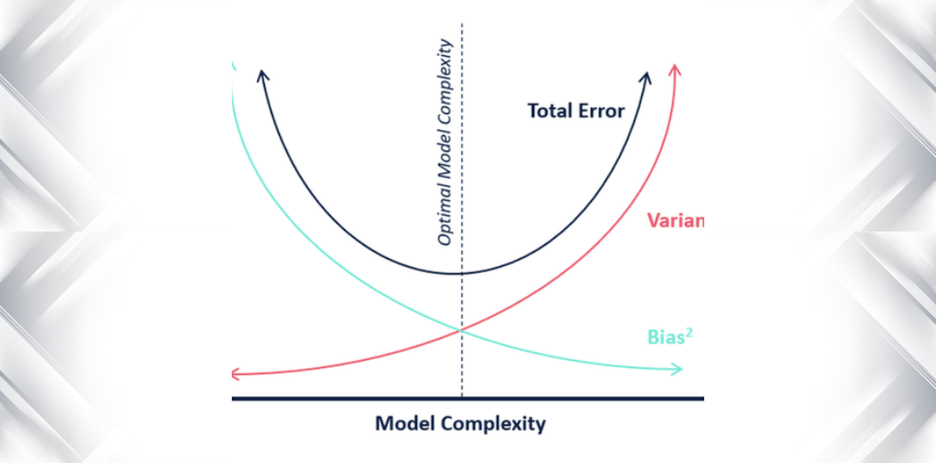
Q31. What is the difference between Variance and Bias in Statistics?

A. In statistics, variance, and bias are two measures of the quality or accuracy of a model or estimator.

• Variance: Variance measures the amount of spread or dispersion in a dataset. It is calculated as the average squared deviation from the mean. A high variance indicates that the data are spread out and may be more prone to error, while a low variance indicates that the data are concentrated around the mean and may be more accurate.
• Bias: Bias refers to the difference between the expected value of an estimator and the true value of the parameter being estimated. A high bias indicates that the estimator is consistently under or overestimating the true value, while a low bias indicates that the estimator is more accurate.

It is important to consider both variance and bias when evaluating the quality of a model or estimator. A model with low bias and high variance may be prone to overfitting, while a model with high bias and low variance may be prone to underfitting. Finding the right balance between bias and variance is an important aspect of model selection and optimization.

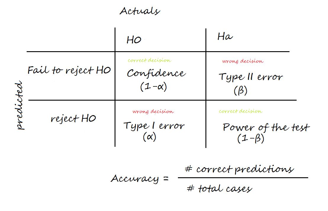
Q32. What is the difference between Type I and Type II errors?

A. Two types of errors can occur in hypothesis testing: Type I errors and Type II errors.

A Type I error, also known as a “false positive,” occurs when the null hypothesis is true but is rejected. This type of error is denoted by the Greek letter alpha (α) and is usually set at a level of 0.05. This means that there is a 5% chance of making a Type I error or a false positive.

A Type II error, also known as a “false negative,” occurs when the null hypothesis is false but is not rejected. This type of error is denoted by the Greek letter beta (β) and is often represented as 1 – β, where β is the power of the test. The power of the test is the probability of correctly rejecting the null hypothesis when it is false.

It’s important to try to minimize the chances of both types of errors in hypothesis testing.

Q33. What is the Confidence Interval in statistics?

A. The confidence interval is the range within which we expect the results to lie if we repeat the experiment. It is the mean of the result plus and minus the expected variation.

The standard error of the estimate determines the latter, while the center of the interval coincides with the mean of the estimate. The most common confidence interval is 95%.

Q34. Can you explain the concept of correlation and covariance?

A. Correlation is a statistical measure that describes the strength and direction of a linear relationship between two variables. A positive correlation indicates that the two variables increase or decrease together, while a negative correlation indicates that the two variables move in opposite directions. Covariance is a measure of the joint variability of two random variables. It is used to measure how two variables are related.

Advanced Statistics Interview Questions

Q35. Why is hypothesis testing useful for a data scientist?

A. Hypothesis testing is a statistical technique used in data science to evaluate the validity of a claim or hypothesis about a population. It is used to determine whether there is sufficient evidence to support a claim or hypothesis and to assess the statistical significance of the results.

There are many situations in data science where hypothesis testing is useful. For example, it can be used to test the effectiveness of a new marketing campaign, to determine if there is a significant difference between the means of two groups, to evaluate the relationship between two variables, or to assess the accuracy of a predictive model.

Hypothesis testing is an important tool in data science because it allows data scientists to make informed decisions based on data, rather than relying on assumptions or subjective opinions. It helps data scientists to draw conclusions about the data that are supported by statistical evidence, and to communicate their findings in a clear and reliable manner. Hypothesis testing is therefore a key component of the scientific method and a fundamental aspect of data science practice.

Q36. What is a chi-square test of independence used for in statistics?

A. A chi-square test of independence is a statistical test used to determine whether there is a significant association between two categorical variables. It is used to test the null hypothesis that the two variables are independent, meaning that the value of one variable does not depend on the value of the other variable.

The chi-square test of independence involves calculating a chi-square statistic and comparing it to a critical value to determine the probability of the observed relationship occurring by chance. If the probability is below a certain threshold (e.g., 0.05), the null hypothesis is rejected and it is concluded that there is a significant association between the two variables.

The chi-square test of independence is commonly used in data science to evaluate the relationship between two categorical variables, such as the relationship between gender and purchasing behavior, or the relationship between education level and voting preference. It is an important tool for understanding the relationship between different variables and for making informed decisions based on the data.

Q37. What is the significance of the p-value?

A. The p-value is used to determine the statistical significance of a result. In hypothesis testing, the p-value is used to assess the probability of obtaining a result that is at least as extreme as the one observed, given that the null hypothesis is true. If the p-value is less than the predetermined level of significance (usually denoted as alpha, α), then the result is considered statistically significant and the null hypothesis is rejected.

The significance of the p-value is that it allows researchers to make decisions about the data based on a predetermined level of confidence. By setting a level of significance before conducting the statistical test, researchers can determine whether the results are likely to have occurred by chance or if there is a real effect present in the data.

Q38.What are the different types of sampling techniques used by data analysts?

A. There are many different types of sampling techniques that data analysts can use, but some of the most common ones include:

• Simple random sampling: This is a basic form of sampling in which each member of the population has an equal chance of being selected for the sample.
• Stratified random sampling: This technique involves dividing the population into subgroups (or strata) based on certain characteristics, and then selecting a random sample from each stratum.
• Cluster sampling: This technique involves dividing the population into smaller groups (or clusters), and then selecting a random sample of clusters. 
• Systematic sampling: This technique involves selecting every kth member of the population to be included in the sample. 

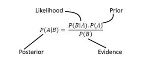
Q39.What is Bayes’ theorem and how is it used in data science?

A. Bayes’ theorem is a mathematical formula that describes the probability of an event occurring, based on prior knowledge of conditions that might be related to the event. In data science, Bayes’ theorem is often used in Bayesian statistics and machine learning, for tasks such as classification, prediction, and estimation.

Q40.What is the difference between a parametric and a non-parametric test?

A. A parametric test is a statistical test that assumes that the data follows a specific probability distribution, such as a normal distribution. A non-parametric test does not make any assumptions about the underlying probability distribution of the data.

Interview Questions Related to Machine Learning

Let us look at data science interview questions and answers regarding Machine Learning.

Beginner ML Interview Questions for Data Science

Q41. What is the difference between feature selection and extraction?

A. Feature selection is the technique in which we filter the features that should be fed to the model. This is the task in which we select the most relevant features. The features that clearly do not hold any importance in determining the prediction of the model are rejected.

Feature selection on the other hand is the process by which the features are extracted from the raw data. It involves transforming raw data into a set of features that can be used to train an ML model. 

Both of these are very important as they help in filtering the features for our ML model which helps in determining the accuracy of the model.

Q42. What are the 5 assumptions for linear regression?

A. Here are the 5 assumptions of linear regression:

• Linearity: There is a linear relationship between the independent variables and the dependent variable.
• Independence of errors: The errors (residuals) are independent of each other.
• Homoscedasticity: The variance of the errors is constant across all predicted values.
• Normality: The errors follow a normal distribution.
• Independence of predictors: The independent variables are not correlated with each other.

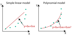
Q43. What is the difference between linear and nonlinear regression?

A.  Linear regression is the method in which is used to find the relationship between a dependent and one or more independent variables. The model finds the best-fit line, which is a linear function (y = mx +c) that helps in fitting the model in such a way that the error is minimum considering all the data points. So the decision boundary of a linear regression function is linear.

A non-Linear regression is used to model the relationship between a dependent and one or more independent variables by a non-linear equation. The non-linear regression models are more flexible and are able to find the more complex relationship between variables.

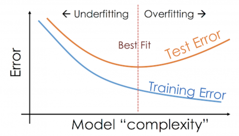
Q44. How will you identify underfitting in a model?

A. Underfitting occurs when a statistical model or machine learning algorithm is not able to capture the underlying trend of the data. This can happen for a variety of reasons, but one common cause is that the model is too simple and is not able to capture the complexity of the data

Here is how to identify underfitting in a model:

The training error of an underfitting error will be high, i.e., the model will not be able to learn from the training data and will perform poorly on the training data.

The validation error of an underfitting model will also be high as it will perform poorly on the new data as well.

Q45. How will you identify overfitting in a model?

A. Overfitting in a model occurs when the model learns the whole training data instead of taking signals/hints from the data and the model performs extremely well on training data and performs poorly on the testing data.

The testing error of the model is high compared to the training error. The bias of an overfitting model is low whereas the variance is high.

Q46. What are some of the techniques to avoid overfitting?

A. Some techniques that can be used to avoid overfitting;

• Train-validation-test split: One way to avoid overfitting is to split your data into training, validation, and test sets. The model is trained on the training set and then evaluated on the validation set. The hyperparameters are then tuned based on the performance on the validation set. Once the model is finalized, it is evaluated on the test set.
• Early stopping: Another way to avoid overfitting is to use early stopping. This involves training the model until the validation error reaches a minimum, and then stopping the training process. 

• Regularization: Regularization is a technique that can be used to prevent overfitting by adding a penalty term to the objective function. This term encourages the model to have small weights, which can help reduce the complexity of the model and prevent overfitting. 
• Ensemble methods: Ensemble methods involve training multiple models and then combining their predictions to make a final prediction. This can help reduce overfitting by averaging out the predictions of the individual models, which can help reduce the variance of the final prediction.

Q47. What are some of the techniques to avoid underfitting?

A. Some techniques to prevent underfitting in a model:

Feature selection: It is important to choose the right feature required for training a model as the selection of the wrong feature can result in underfitting.

Increasing the number of features helps to avoid underfitting

Using a more complex machine-learning model

Using Hyperparameter tuning to fine tune the parameters in the model

Noise: If there is more noise in the data, the model will not be able to detect the complexity of the dataset.

Q48. What is Multicollinearity?

A. Multicollinearity occurs when two or more predictor variables in a multiple regression model are highly correlated. This can lead to unstable and inconsistent coefficients, and make it difficult to interpret the results of the model.

In other words, multicollinearity occurs when there is a high degree of correlation between two or more predictor variables. This can make it difficult to determine the unique contribution of each predictor variable to the response variable, as the estimates of their coefficients may be influenced by the other correlated variables.

Q49. Explain regression and classification problems.

A. Regression is a method of modeling the relationship between one or more independent variables and a dependent variable. The goal of regression is to understand how the independent variables are related to the dependent variable and to be able to make predictions about the value of the dependent variable based on new values of the independent variables.

A classification problem is a type of machine learning problem where the goal is to predict a discrete label for a given input. In other words, it is a problem of identifying to which set of categories a new observation belongs, on the basis of a training set of data containing observations.

Q50. What is the difference between K-means and KNN?

A. K-means and KNN (K-Nearest Neighbors) are two different machine learning algorithms.

K-means is a clustering algorithm that is used to divide a group of data points into K clusters, where each data point belongs to the cluster with the nearest mean. It is an iterative algorithm that assigns data points to a cluster and then updates the cluster centroid (mean) based on the data points assigned to it.

On the other hand, KNN is a classification algorithm that is used to classify data points based on their similarity to other data points. It works by finding the K data points in the training set that are most similar to the data point being classified, and then it assigns the data point to the class that is most common among those K data points.

So, in summary, K-means is used for clustering, and KNN is used for classification.

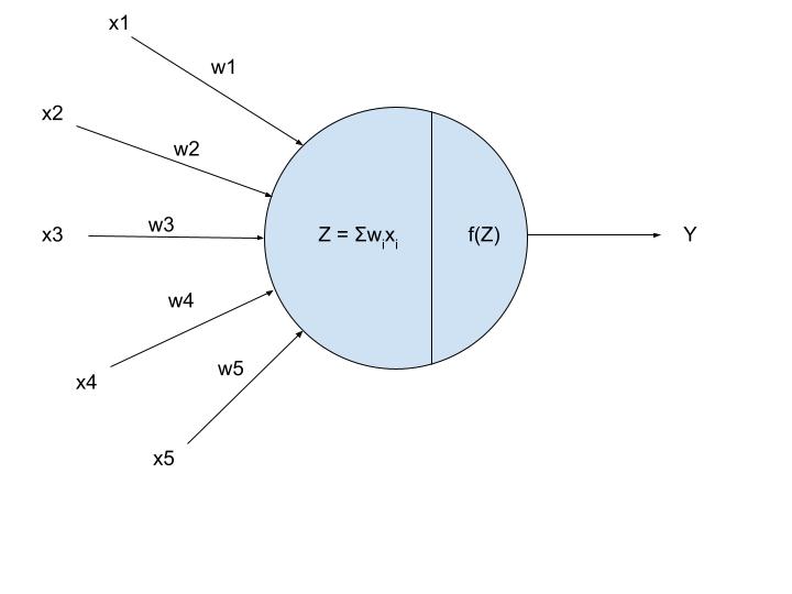
Q51. What is the difference between Sigmoid and Softmax ?

A. In Sigmoid function if your output is binary (0,1) then use the sigmoid function for the output layer. The sigmoid function appears in the output layer of the deep learning models and is used for predicting probability-based outputs.

The softmax function is another type of Activation Function used in neural networks to compute probability distribution from a vector of real numbers.

This function is mainly used in multi-class models where it returns probabilities of each class, with the target class having the highest probability.

The primary difference between the sigmoid and softmax Activation function is that while the former is used in binary classification, the latter is used for multivariate classification

Q52. Can we use logistic regression for multiclass classification?

A. Yes, logistic regression can be used for multiclass classification.

Logistic regression is a classification algorithm that is used to predict the probability of a data point belonging to a certain class. It is a binary classification algorithm, which means that it can only handle two classes. However, there are ways to extend logistic regression to multiclass classification.

One way to do this is to use one-vs-all (OvA) or one-vs-rest (OvR) strategy, where you train K logistic regression classifiers, one for each class, and assign a data point to the class that has the highest predicted probability. This is called OvA if you train one classifier for each class, and the other class is the “rest” of the classes. This is called OvR if you train one classifier for each class, and the other class is the “all” of the classes.

Another way to do this is to use multinomial logistic regression, which is a generalization of logistic regression to the case where you have more than two classes. In multinomial logistic regression, you train a logistic regression classifier for each pair of classes, and you use the predicted probabilities to assign a data point to the class that has the highest probability.

So, in summary, logistic regression can be used for multiclass classification using OvA/OvR or multinomial logistic regression.

Q53. Can you explain the bias-variance tradeoff in the context of supervised machine learning?

A. In supervised machine learning, the goal is to build a model that can make accurate predictions on unseen data. However, there is a tradeoff between the model’s ability to fit the training data well (low bias) and its ability to generalize to new data (low variance).

A model with high bias tends to underfit the data, which means that it is not flexible enough to capture the patterns in the data. On the other hand, a model with high variance tends to overfit the data, which means that it is too sensitive to noise and random fluctuations in the training data.

The bias-variance tradeoff refers to the tradeoff between these two types of errors. A model with low bias and high variance is likely to overfit the data, while a model with high bias and low variance is likely to underfit the data.

To balance the tradeoff between bias and variance, we need to find a model with the right complexity level for the problem at hand. If the model is too simple, it will have high bias and low variance, but it will not be able to capture the underlying patterns in the data. If the model is too complex, it will have low bias and high variance, but it will be sensitive to the noise in the data and it will not generalize well to new data.

Q54. How do you decide whether a model is suffering from high bias or high variance?

A. There are several ways to determine whether a model is suffering from high bias or high variance. Some common methods are:

Split the data into a training set and a test set, and check the performance of the model on both sets. If the model performs well on the training set but poorly on the test set, it is likely to suffer from high variance (overfitting). If the model performs poorly on both sets, it is likely suffering from high bias (underfitting).

Use cross-validation to estimate the performance of the model. If the model has high variance, the performance will vary significantly depending on the data used for training and testing. If the model has high bias, the performance will be consistently low across different splits of the data.

Plot the learning curve, which shows the performance of the model on the training set and the test set as a function of the number of training examples. A model with high bias will have a high training error and a high test error, while a model with high variance will have a low training error and a high test error.

Q55. What are some techniques for balancing bias and variance in a model?

A. There are several techniques that can be used to balance the bias and variance in a model, including:

Increasing the model complexity by adding more parameters or features: This can help the model capture more complex patterns in the data and reduce bias, but it can also increase variance if the model becomes too complex.

Reducing the model complexity by removing parameters or features: This can help the model avoid overfitting and reduce variance, but it can also increase bias if the model becomes too simple.

Using regularization techniques: These techniques constrain the model complexity by penalizing large weights, which can help the model avoid overfitting and reduce variance. Some examples of regularization techniques are L1 regularization, L2 regularization, and elastic net regularization.

Splitting the data into a training set and a test set: This allows us to evaluate the model’s generalization ability and tune the model complexity to achieve a good balance between bias and variance.

Using cross-validation: This is a technique for evaluating the model’s performance on different splits of the data and averaging the results to get a more accurate estimate 

of the model’s generalization ability.

Q56. How do you choose the appropriate evaluation metric for a classification problem, and how do you interpret the results of the evaluation?

A. There are many evaluation metrics that you can use for a classification problem, and the appropriate metric depends on the specific characteristics of the problem and the goals of the evaluation. Some common evaluation metrics for classification include:

• Accuracy: This is the most common evaluation metric for classification. It measures the percentage of correct predictions made by the model.
• Precision: This metric measures the proportion of true positive predictions among all positive predictions made by the model.
• Recall: This metric measures the proportion of true positive predictions among all actual positive cases in the test set.
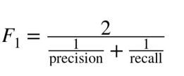
• F1 Score: This is the harmonic mean of precision and recall. It is a good metric to use when you want to balance precision and recall.
• AUC-ROC: This metric measures the ability of the model to distinguish between positive and negative classes. It is commonly used for imbalanced classification problems.

To interpret the results of the evaluation, you should consider the specific characteristics of the problem and the goals of the evaluation. For example, if you are trying to identify fraudulent transactions, you may be more interested in maximizing precision, because you want to minimize the number of false alarms. On the other hand, if you are trying to diagnose a disease, you may be more interested in maximizing recall, because you want to minimize the number of missed diagnoses.

Q57. What is the difference between K-means and hierarchical clustering and when to use what?

A. K-means and hierarchical clustering are two different methods for clustering data. Both methods can be useful in different situations.

K-means is a centroid-based algorithm, or a distance-based algorithm, where we calculate the distances to assign a point to a cluster. K-means is very fast and efficient in terms of computational time, but it can fail to find the global optimum because it uses random initializations for the centroid seeds.

Hierarchical clustering, on the other hand, is a density-based algorithm that does not require us to specify the number of clusters beforehand. It builds a hierarchy of clusters by creating a tree-like diagram, called a dendrogram. There are two main types of hierarchical clustering: agglomerative and divisive. Agglomerative clustering starts with individual points as separate clusters and merges them into larger clusters, while divisive clustering starts with all points in one cluster and divides them into smaller clusters. Hierarchical clustering is a slow algorithm and requires a lot of computational resources, but it is more accurate than K-means.

So, when to use K-means and when to use hierarchical clustering? It really depends on the size and structure of your data, as well as the resources you have available. If you have a large dataset and you want to cluster it quickly, then K-means might be a good choice. If you have a small dataset or if you want more accurate clusters, then hierarchical clustering might be a better choice.

Q58. How can you handle imbalanced classes in a logistic regression model?

A. There are several ways to handle imbalanced classes in a logistic regression model. Some approaches include:

• Undersampling the majority class: This involves randomly selecting a subset of the majority class samples to use in training the model. This can help to balance the class distribution, but it may also throw away valuable information.
• Oversampling the minority class: This involves generating synthetic samples of the minority class to add to the training set. One popular method for generating synthetic samples is called SMOTE (Synthetic Minority Oversampling Technique).
• Adjusting the class weights: Many machine learning algorithms allow you to adjust the weighting of each class. In logistic regression, you can do this by setting the class_weight parameter to “balanced”. This will automatically weight the classes inversely proportional to their frequency, so that the model pays more attention to the minority class.
• Using a different evaluation metric: In imbalanced classification tasks, it is often more informative to use evaluation metrics that are sensitive to class imbalance, such as precision, recall, and the F1 score.
• Using a different algorithm: Some algorithms, such as decision trees and Random Forests, are more robust to imbalanced classes and may perform better on imbalanced datasets.

Q59. When not to use PCA for dimensionality reduction?

A. There are several situations when you may not want to use Principal Component Analysis (PCA) for dimensionality reduction:

When the data is not linearly separable: PCA is a linear technique, so it may not be effective at reducing the dimensionality of data that is not linearly separable.

The data has categorical features: PCA is designed to work with continuous numerical data and may not be effective at reducing the dimensionality of data with categorical features.

When the data has a large number of missing values: PCA is sensitive to missing values and may not work well with data sets that have a large number of missing values.

The goal is to preserve the relationships between the original features: PCA is a technique that looks for patterns in the data and creates new features that are combinations of the original features. As a result, it may not be the best choice if the goal is to preserve the relationships between the original features.

When the data is highly imbalanced: PCA is sensitive to class imbalances and may not produce good results on highly imbalanced data sets.

Q60. What is Gradient descent?

A. Gradient descent is an optimization algorithm used in machine learning to find the values of parameters (coefficients and bias) of a model that minimize the cost function. It is a first-order iterative optimization algorithm that follows the negative gradient of the cost function to converge to the global minimum.

In gradient descent, the model’s parameters are initialized with random values, and the algorithm iteratively updates the parameters in the opposite direction of the gradient of the cost function with respect to the parameters. The size of the update is determined by the learning rate, which is a hyperparameter that controls how fast the algorithm converges to the global minimum.

As the algorithm updates the parameters, the cost function decreases and the model’s performance improves

Q61. What is the difference between MinMaxScaler and StandardScaler?

A. Both the MinMaxScaler and StandardScaler are tools used to transform the features of a dataset so that they can be better modeled by machine learning algorithms. However, they work in different ways.

MinMaxScaler scales the features of a dataset by transforming them to a specific range, usually between 0 and 1. It does this by subtracting the minimum value of each feature from all the values in that feature, and then dividing the result by the range (i.e., the difference between the minimum and maximum values). This transformation is given by the following equation:

x_scaled = (x - x_min) / (x_max - x_min)

StandardScaler standardizes the features of a dataset by transforming them to have zero mean and unit variance. It does this by subtracting the mean of each feature from all the values in that feature, and then dividing the result by the standard deviation. This transformation is given by the following equation:

x_scaled = (x - mean(x)) / std(x)

In general, StandardScaler is more suitable for datasets where the distribution of the features is approximately normal, or Gaussian. MinMaxScaler is more suitable for datasets where the distribution is skewed or where there are outliers. However, it is always a good idea to visualize the data and understand the distribution of the features before choosing a scaling method.

Q62. What is the difference between Supervised and Unsupervised learning?

A. In supervised learning, the training set you feed to the algorithm includes the desired solutions, called labels.

Ex = Spam Filter (Classification problem)

k-Nearest Neighbors

• Linear Regression
• Logistic Regression
• Support Vector Machines (SVMs)
• Decision Trees and Random Forests
• Neural networks

In unsupervised learning, the training data is unlabeled.

Let’s say, The system tries to learn without a teacher.

• Clustering
  • K-Means
  • DBSCAN
  • Hierarchical Cluster Analysis (HCA)
• Anomaly detection and novelty detection
  • One-class SVM
  • Isolation Forest
• Visualization and dimensionality reduction
  • Principal Component Analysis (PCA)
  • Kernel PCA
  • Locally Linear Embedding (LLE)
  • t-Distributed Stochastic Neighbor Embedding (t-SNE)

Q63. What are some common methods for hyperparameter tuning?

A. There are several common methods for hyperparameter tuning:

• Grid Search: This involves specifying a set of values for each hyperparameter, and the model is trained and evaluated using a combination of all possible hyperparameter values. This can be computationally expensive, as the number of combinations grows exponentially with the number of hyperparameters.
• Random Search: This involves sampling random combinations of hyperparameters and training and evaluating the model for each combination. This is less computationally intensive than grid search, but may be less effective at finding the optimal set of hyperparameters.

Q64. How do you decide the size of your validation and test sets?

A. You can validate the size of your test sets in the following ways:

• Size of the dataset: In general, the larger the dataset, the larger the validation and test sets can be. This is because there is more data to work with, so the validation and test sets can be more representative of the overall dataset.
• Complexity of the model: If the model is very simple, it may not require as much data to validate and test. On the other hand, if the model is very complex, it may require more data to ensure that it is robust and generalizes well to unseen data.
• Level of uncertainty: If the model is expected to perform very well on the task, the validation and test sets can be smaller. However, if the performance of the model is uncertain or the task is very challenging, it may be helpful to have larger validation and test sets to get a more accurate assessment of the model’s performance.
• Resources available: The size of the validation and test sets may also be limited by the computational resources available. It may not be practical to use very large validation and test sets if it takes a long time to train and evaluate the model.

Q65. How do you evaluate a model’s performance for a multi-class classification problem?

A. One approach for evaluating a multi-class classification model is to calculate a separate evaluation metric for each class, and then calculate a macro or micro average. The macro average gives equal weight to all the classes, while the micro average gives more weight to the classes with more observations. Additionally, some commonly used metrics for multi-class classification problems such as confusion matrix, precision, recall, F1 score, Accuracy and ROC-AUC can also be used.

Q66. What is the difference between Statistical learning and Machine Learning with their examples?

A. Statistical learning and machine learning are both methods used to make predictions or decisions based on data. However, there are some key differences between the two approaches:

Statistical learning focuses on making predictions or decisions based on a statistical model of the data. The goal is to understand the relationships between the variables in the data and make predictions based on those relationships. Machine learning, on the other hand, focuses on making predictions or decisions based on patterns in the data, without necessarily trying to understand the relationships between the variables.

Statistical learning methods often rely on strong assumptions about the data distribution, such as normality or independence of errors. Machine learning methods, on the other hand, are often more robust to violations of these assumptions.

Statistical learning methods are generally more interpretable because the statistical model can be used to understand the relationships between the variables in the data. Machine learning methods, on the other hand, are often less interpretable, because they are based on patterns in the data rather than explicit relationships between variables.

For example, linear regression is a statistical learning method that assumes a linear relationship between the predictor and target variables and estimates the coefficients of the linear model using an optimization algorithm. Random forests is a machine learning method that builds an ensemble of decision trees and makes predictions based on the average of the predictions of the individual trees. 

Q67. How is normalized data beneficial for making models in data science?

A. Improved model performance: Normalizing the data can improve the performance of some machine learning models, particularly those that are sensitive to the scale of the input data. For example, normalizing the data can improve the performance of algorithms such as K-nearest neighbors and neural networks.

• Easier feature comparison: Normalizing the data can make it easier to compare the importance of different features. Without normalization, features with large scales can dominate the model, making it difficult to determine the relative importance of other features.
• Reduced impact of outliers: Normalizing the data can reduce the impact of outliers on the model, as they are scaled down along with the rest of the data. This can improve the robustness of the model and prevent it from being influenced by extreme values.
• Improved interpretability: Normalizing the data can make it easier to interpret the results of the model, as the coefficients and feature importances are all on the same scale.

It is important to note that normalization is not always necessary or beneficial for all models. It is necessary to carefully evaluate the specific characteristics and needs of the data and the model in order to determine whether normalization is appropriate.

Intermediate ML Interview Questions

Q68. Why is the harmonic mean calculated in the f1 score and not the mean?

A. The F1 score is a metric that combines precision and recall. Precision is the number of true positive results divided by the total number of positive results predicted by the classifier, and recall is the number of true positive results divided by the total number of positive results in the ground truth. The harmonic mean of precision and recall is used to calculate the F1 score because it is more forgiving of imbalanced class proportions than the arithmetic mean.

If the harmonic means were not used, the F1 score would be higher because it would be based on the arithmetic mean of precision and recall, which would give more weight to the high precision and less weight to the low recall. The use of the harmonic mean in the F1 score helps to balance the precision and recall and gives a more accurate overall assessment of the classifier’s performance.

Q69. What are some ways to select features?

A. Here are some ways to select the features:

• Filter methods: These methods use statistical scores to select the most relevant features. 

Example:

• Correlation coefficient: Selects features that are highly correlated with the target variable.
• Chi-squared test: Selects features that are independent of the target variable.
• Wrapper methods: These methods use a learning algorithm to select the best features. 

For example

• Forward selection: Begins with an empty set of features and adds one feature at a time until the performance of the model is optimal.
• Backward selection: Begins with the full set of features and removes one feature at a time until the performance of the model is optimal.
• Embedded methods: These methods learn which features are most important while the model is being trained.

Example:

• Lasso regression: Regularizes the model by adding a penalty term to the loss function that shrinks the coefficients of the less important features to zero.
• Ridge regression: Regularizes the model by adding a penalty term to the loss function that shrinks the coefficients of all features towards zero, but does not set them to zero.
• Feature Importance: We can also use the feature importance parameter which gives us the most important features considered by the model

Q70. What is the difference between bagging boosting difference?

A. Both bagging and boosting are ensemble learning techniques that help in improving the performance of the model.

Bagging is the technique in which different models are trained on the dataset that we have and then the average of the predictions of these models is taken into consideration. The intuition behind taking the predictions of all the models and then averaging the results is making more diverse and generalized predictions that can be more accurate.

Boosting is the technique in which different models are trained but they are trained in a sequential manner. Each successive model corrects the error made by the previous model. This makes the model strong resulting in the least error.

Q71. What is the difference between stochastic gradient boosting and XGboost?

A. XGBoost is an implementation of gradient boosting that is specifically designed to be efficient, flexible, and portable. Stochastic XGBoost is a variant of XGBoost that uses a more randomized approach to building decision trees, which can make the resulting model more robust to overfitting. 

Both XGBoost and stochastic XGBoost are popular choices for building machine-learning models and can be used for a wide range of tasks, including classification, regression, and ranking. The main difference between the two is that XGBoost uses a deterministic tree construction algorithm, while stochastic XGBoost uses a randomized tree construction algorithm.

Q72. What is the difference between catboost and XGboost?

A. Difference between Catboost and XGboost:

• Catboost handles categorical features better than XGboost. In catboost, the categorical features are not required to be one-hot encoded which saves a lot of time and memory. XGboost on the other hand can also handle categorical features but they needed to be one-hot encoded first.
• XGboost requires manual processing of the data while Catboost does not. They have some differences in the way that they build decision trees and make predictions.

Catboost is faster than XGboost and builds symmetric(balanced) trees, unlike XGboost.

Q73. What is the difference between linear and nonlinear classifiers

A. The difference between the linear and nonlinear classifiers is the nature of the decision boundary.

In a linear classifier, the decision boundary is a linear function of the input. In other words, the boundary is a straight line, a plane, or a hyperplane. 

ex: Linear Regression, Logistic Regression, LDA

A non-linear classifier is one in which the decision boundary is not a linear function of the input.  This means that the classifier cannot be represented by a linear function of the input features. Non-linear classifiers can capture more complex relationships between the input features and the label, but they can also be more prone to overfitting, especially if they have a lot of parameters.

ex: KNN, Decision Tree, Random Forest

Q74. What are parametric and nonparametric models?

A. A parametric model is a model that is described by a fixed number of parameters. These parameters are estimated from the data using a maximum likelihood estimation procedure or some other method, and they are used to make predictions about the response variable.

Nonparametric models do not assume any specific form for the relationship between variables. They are more flexible than parametric models. They can fit a wider variety of data shapes. However, they have fewer interpretable parameters. This can make them harder to understand.

Q75. How can we use cross-validation to overcome overfitting?

A. The cross-validation technique can be used to identify if the model is underfitting or overfitting but it cannot be used to overcome either of the problems. We can only compare the performance of the model on two different sets of data and find if the data is overfitting or underfitting, or generalized.

Q76. How can you convert a numerical variable to a categorical variable and when can it be useful?

A. There are several ways to convert a numerical variable to a categorical variable. One common method is to use binning, which involves dividing the numerical variable into a set of bins or intervals and treating each bin as a separate category.

Another way to convert a numerical variable to a categorical one is through “discretization.” This means dividing the range into intervals. Each interval is then treated as a separate category. It helps create a more detailed view of the data.

This conversion is useful when the numerical variable has limited values. Grouping these values can make patterns clearer. It also highlights trends instead of focusing on raw numbers.

Q77. What are generalized linear models?

A. Generalized Linear Models are a flexible family of models. They describe the relationship between a response variable and one or more predictors. GLMs offer more flexibility than traditional linear models.

In linear models, the response is normally distributed. The relationship with predictors is assumed to be linear. GLMs relax these rules. The response can follow different distributions. The relationship can also be non-linear. Common GLMs include logistic regression for binary data, Poisson regression for counts, and exponential regression for time-to-event data.

Q78. What is the difference between ridge and lasso regression? How do they differ in terms of their approach to model selection and regularization?

A. Ridge regression and lasso regression are both techniques used to prevent overfitting in linear models by adding a regularization term to the objective function. They differ in how they define the regularization term.

In ridge regression, the regularization term is defined as the sum of the squared coefficients (also called the L2 penalty). This results in a smooth optimization surface, which can help the model generalize better to unseen data. Ridge regression has the effect of driving the coefficients towards zero, but it does not set any coefficients exactly to zero. This means that all features are retained in the model, but their impact on the output is reduced.

On the other hand, lasso regression defines the regularization term as the sum of the absolute values of the coefficients (also called the L1 penalty). This has the effect of driving some coefficients exactly to zero, effectively selecting a subset of the features to use in the model. This can be useful for feature selection, as it allows the model to automatically select the most important features. However, the optimization surface for lasso regression is not smooth, which can make it more difficult to train the model.

In summary, ridge regression shrinks the coefficients of all features towards zero, while lasso regression sets some coefficients exactly to zero. Both techniques can be useful for preventing overfitting, but they differ in how they handle model selection and regularization.

Q79.How does the step size (or learning rate) of an optimization algorithm impact the convergence of the optimization process in logistic regression?

A. The step size, or learning rate, controls how big the steps are during optimization. In logistic regression, we minimize the negative log-likelihood to find the best coefficients. If the step size is too large, the algorithm may overshoot the minimum. It can oscillate or even diverge. If the step size is too small, progress will be slow. The algorithm may take a long time to converge.

Therefore, it is important to choose an appropriate step size in order to ensure the convergence of the optimization process. In general, a larger step size can lead to faster convergence, but it also increases the risk of overshooting the minimum. A smaller step size will be safer, but it will also be slower.

There are several approaches for choosing an appropriate step size. One common approach is to use a fixed step size for all iterations. Another approach is to use a decreasing step size, which starts out large and decreases over time. This can help the optimization algorithm to make faster progress at the beginning and then fine-tune the coefficients as it gets closer to the minimum.

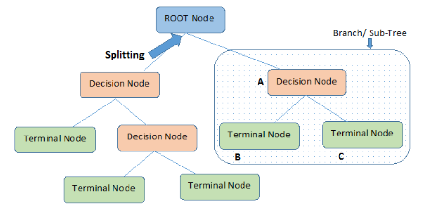
Q80. What is overfitting in decision trees, and how can it be mitigated?

A. Overfitting in decision trees occurs when the model is too complex and has too many branches, leading to poor generalization to new, unseen data. This is because the model has “learned” the patterns in the training data too well, and is not able to generalize these patterns to new, unseen data.

There are several ways to mitigate overfitting in decision trees:

• Pruning: This involves removing branches from the tree that do not add significant value to the model’s predictions. Pruning can help reduce the complexity of the model and improve its generalization ability.
• Limiting tree depth: By restricting the depth of the tree, you can prevent the tree from becoming too complex and overfitting the training data.
• Using ensembles: Ensemble methods such as random forests and gradient boosting can help reduce overfitting by aggregating the predictions of multiple decision trees.
• Using cross-validation: By evaluating the model’s performance on multiple train-test splits, you can get a better estimate of the model’s generalization performance and reduce the risk of overfitting.

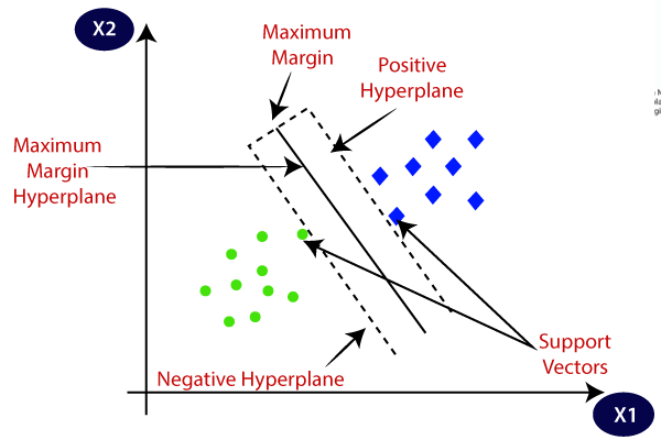
Q81. Why is SVM called a large margin classifier?

A. Support Vector Machine, is called a large margin classifier because it seeks to find a hyperplane with the largest possible margin, or distance, between the positive and negative classes in the feature space. The margin is the distance between the hyperplane and the nearest data points, and is used to define the decision boundary of the model.

By maximizing the margin, the SVM classifier is able to better generalize to new, unseen data and is less prone to overfitting. The larger the margin, the lower the uncertainty around the decision boundary, and the more confident the model is in its predictions.

Therefore, the goal of the SVM algorithm is to find a hyperplane with the largest possible margin, which is why it is called a large margin classifier.

Q82. What is hinge loss?

A. Hinge loss is a loss function used in support vector machines (SVMs) and other linear classification models. It is defined as the loss that is incurred when a prediction is incorrect.

The hinge loss for a single example is defined as:

loss = max(0, 1 – y * f(x))

where y is the true label (either -1 or 1) and f(x) is the predicted output of the model. The predicted output is the inner product between the input features and the model weights, plus a bias term.

Hinge loss is used in SVMs because it is convex. It penalizes predictions that are not confident and correct. The loss is zero when the prediction is correct. It increases as confidence in a wrong prediction grows. This pushes the model to be confident but careful. It discourages predictions far from the true label.

Advanced ML Interview Questions

Q83. What will happen if we increase the number of neighbors in KNN?

A. Increasing the number of neighbors in KNN makes the classifier more conservative. The decision boundary becomes smoother. This helps reduce overfitting. However, it may miss subtle patterns in the data. A larger k creates a simpler model. This lowers overfitting but increases the risk of underfitting.

To avoid both issues, choosing the right k is important. It should balance complexity and simplicity. It’s best to test different k values. Then, pick the one that works best for your dataset.

Q84. What will happen in the decision tree if the max depth is increased?

A. Increasing the max depth of a decision tree will increase the complexity of the model and make it more prone to overfitting. If you increase the max depth of a decision tree, the tree will be able to make more complex and nuanced decisions, which can improve the model’s ability to fit the training data well. However, if the tree is too deep, it may become overly sensitive to the specific patterns in the training data and not generalize well to unseen data.

Q85. What is the difference between extra trees and random forests?

A. The main difference between the two algorithms is how the decision trees are constructed.

In a Random Forest, the decision trees are constructed using bootstrapped samples of the training data and a random subset of the features. This results in each tree being trained on a slightly different set of data and features, leading to a greater diversity of trees and a lower variance.

In an Extra Trees classifier, the decision trees are constructed in a similar way, but instead of selecting a random subset of the features at each split, the algorithm selects the best split among a random subset of the features. This results in a greater number of random splits and a higher degree of randomness, leading to a lower bias and a higher variance.

Q86. When to use one-hot encoding and label encoding?

A. One-hot encoding and label encoding are two different techniques that can be used to encode categorical variables as numerical values. They are often used in machine learning models as a preprocessing step before fitting the model to the data.

One-hot encoding is used for categorical variables without any natural order. It creates binary columns for each category, using 1 for presence and 0 for absence, helping preserve uniqueness and avoid false ordinal assumptions. Label encoding is used when categories have a natural order, assigning each a unique integer to reflect that order. One-hot suits nominal data, while label encoding fits ordinal data, though the final choice depends on the model and dataset.

Q87. What is the problem with using label encoding for nominal data?

A. Label encoding is a method of encoding categorical variables as numerical values, which can be beneficial in certain situations. However, there are some potential problems that you should be aware of when using label encoding for nominal data.

One problem with label encoding is that it can create an ordinal relationship between categories where none exists

If you have a categorical variable with three categories: “red”, “green”, and “blue”, and you apply label encoding to map these categories to numerical values 0, 1, and 2, the model may assume that the category “green” is somehow “between” the categories “red” and “blue”. This can be a problem if your model depends on the assumption that the categories are independent of one another.

Another problem with label encoding is that it can lead to unexpected results if you have an imbalanced dataset. For example, if one category is much more common than the others, it will be assigned a much lower numerical value, which could lead the model to give it less importance than it deserves.

Q88. When can one-hot encoding be a problem?

A. One-hot encoding can be a problem in certain situations because it can create a large number of new columns in the dataset, which can make the data more difficult to work with and potentially lead to overfitting.

One-hot encoding creates a new binary column for each category in a categorical variable. If you have a categorical variable with many categories, this can result in a very large number of new columns.

Another problem with one-hot encoding is that it can lead to overfitting. Especially if you have a small dataset and a large number of categories. When you create many new columns for each category, you are effectively increasing the number of features in the dataset. This can lead to overfitting, because the model may be able to memorize the training data, but it will not generalize well to new data.

Finally, one-hot encoding can also be a problem if you need to add new categories to the dataset in the future. If you have already one-hot encoded the existing categories. Ensure new categories are added clearly to avoid confusion or unexpected results.

Q89. What can be an appropriate encoding technique when you have hundreds of categorical values in a column?

A. A few techniques can be used when we have hundreds of columns in a categorical variable.

Frequency encoding: This involves replacing each category with the frequency of that category in the dataset. This can work well if the categories have a natural ordinal relationship based on their frequency.

Target encoding: This involves replacing each category with the mean of the target variable for that category. This can be effective if the categories have a clear relationship with the target variable.

Q90. What are the sources of randomness in random forest ?

A. Random forests are an ensemble learning method that involves training multiple decision trees on different subsets of the data and averaging the predictions of the individual trees to make a final prediction. There are several sources of randomness in the process of training a random forest:

• Bootstrapped samples: When training each decision tree, the algorithm creates a bootstrapped sample of the data by sampling with replacement from the original training set. This means that some data points will be included in the sample multiple times. While others will not be included at all. This creates variation between the training sets of different trees.
• Random feature selection: When training each decision tree, the algorithm selects a random subset of the features to consider at each split. This means that different trees will consider different sets of features, leading to variation in the learned trees.
• Random threshold selection: When training each decision tree, the algorithm selects a random threshold for each feature to determine the optimal split. This means that different trees will split on different thresholds, leading to variation in the learned trees.

Q91. How do you decide which feature to split on at each node of the tree?

A. When training a decision tree, the algorithm must choose the feature to split on at each node of the tree. There are several strategies that can be used to decide which feature to split on, including:

• Greedy search: The algorithm selects the feature that maximizes a splitting criterion (such as information gain or Gini impurity) at each step.
• Random Search: The algorithm selects the feature to split on at random at each step.
• Exhaustive search: The algorithm considers all possible splits and selects the one that maximizes the splitting criterion.
• Forward search: The algorithm starts with an empty tree and adds splits one by one, selecting the split that maximizes the splitting criterion at each step.
• Backward search: The algorithm starts with a fully grown tree and prunes split one by one, selecting the split to remove that results in the smallest decrease in the splitting criterion.

Q92. What is the significance of C in SVM?

A. In the support vector machine (SVM) algorithm, the parameter C is a hyperparameter that controls the trade-off between maximizing the margin and minimizing the misclassification error.

C controls the penalty for misclassifying training examples. A smaller C means a higher penalty. The model tries to classify all examples correctly, even with a smaller margin. A larger C means a lower penalty. The model allows some misclassifications to get a larger margin.

In practice, you can think of C as controlling the flexibility of the model. A smaller value of C will result in a more rigid model that may be more prone to underfitting, while a larger value of C will result in a more flexible model that may be more prone to overfitting.

Choose C carefully using cross-validation to balance bias-variance and ensure good performance on unseen data.

Q93. How do c and gamma affect overfitting in SVM?

A. In support vector machines (SVMs), the regularization parameter C and the kernel parameter gamma are used to control overfitting.

C is the penalty for misclassification. A smaller value of C means a larger penalty for misclassification. The model becomes more conservative. It tries harder to avoid mistakes. This can reduce overfitting. However, it may also make the model too cautious. As a result, generalization performance might suffer.

Gamma is a parameter that controls the complexity of the model. A smaller value of gamma means a more complex model, which can lead to overfitting. A larger value of gamma means a simpler model, which can help prevent overfitting but may also result in a model that is too simple to accurately capture the underlying relationships in the data.

Finding the best values for C and gamma is a balance between bias and variance. It usually requires testing different values. The model’s performance should be checked on a validation set. This helps identify the best parameter settings.

Q94. How do you choose the number of models to use in a Boosting or Bagging ensemble?

A. The number of models to use in an ensemble is usually determined by the trade-off between performance and computational cost. As a general rule of thumb, increasing the number of models will improve the performance of the ensemble, but at the cost of increasing the computational cost.

In practice, the number of models is determined by Cross validation which is used to determine the optimal number of models based on the evaluation metric chosen.

Q95. In which scenarios Boosting and Bagging are preferred over single models?

A. Both boosting and bagging are used to improve model performance. They help when individual models have high variance or high bias. Bagging reduces the variance of a model. Boosting reduces bias and improves generalization error. Both methods are useful for models that are sensitive to training data. They also help when there is a high risk of overfitting.

Q96. Can you explain the ROC curve and AUC score and how they are used to evaluate a model’s performance?

A. A ROC (Receiver Operating Characteristic) curve is a graphical representation of the performance of a binary classification model. It plots the true positive rate (TPR) against the false positive rate (FPR) at different thresholds. AUC (Area Under the Curve) is the area under the ROC curve. It gives a single number that represents the model’s overall performance. AUC is useful because it considers all possible thresholds, not just a single point on the ROC curve.

Q97. How do you approach setting the threshold in a binary classification problem when you want to adjust precision and recall by yourself?

A. When setting the threshold in a binary classification problem, it’s important to consider the trade-off between precision and recall. Precision is the ratio of true positives to all predicted positives. Recall is the ratio of true positives to all actual positives. To adjust these metrics, first train the model and evaluate it on a validation set. This set should have a similar distribution to the test data. Then, use a confusion matrix to visualize performance. It shows true positives, false positives, true negatives, and false negatives. This helps identify the current prediction threshold.

Once you know the threshold, you can adjust it to balance precision and recall. Increasing the threshold boosts precision but lowers recall. Decreasing it raises recall but reduces precision. Always consider the specific use case. In medical diagnosis, high recall is vital to catch all positives. In fraud detection, high precision is key to avoid false alarms. The right balance depends on the cost of false positives and false negatives in your scenario.

Q98. What is the difference between LDA (Linear Discriminant Analysis) and PCA (Principal Component Analysis)?

A. The difference between LDA (Linear Discriminant Analysis) and PCA (Principal Component Analysis) are:

Feature	PCA (Principal Component Analysis)	LDA (Linear Discriminant Analysis)
Type	Unsupervised	Supervised
Purpose	Find directions of maximum variance in the data	Maximize class separability
Use Case	Pattern discovery, data compression	Classification tasks (e.g., face, iris, fingerprint recognition)
Based On	Variance in data	Labels and class distribution
Components	Principal components (orthogonal directions of maximum variance)	Linear discriminants (directions that best separate classes)
Data Projection	Projects data onto directions of highest variance	Projects data onto directions that best separate the classes
Orthogonality	Components are mutually orthogonal	Components are not necessarily orthogonal
Output	Lower-dimensional subspace preserving most variance	Lower-dimensional subspace maximizing class discrimination

Q99. How does the Naive Bayes algorithm compare to other supervised learning algorithms?

A. Naive Bayes is a simple and fast algorithm that works well with high-dimensional data and small training sets. It also performs well on datasets with categorical variables and missing data, which are common in many real-world problems. It is good for text classification, spam filtering, and sentiment analysis. However, due to the assumption of independence among features, it does not perform good for problems having high correlation among features. It also often fails to capture the interactions among features, which can result in poor performance on some datasets. Therefore, it is often used as a baseline or starting point, and then other algorithms like SVM, and Random Forest can be used to improve the performance.

Q100. Can you explain the concept of the “kernel trick” and its application in Support Vector Machines (SVMs)?

A. The kernel trick is a technique used in SVMs. It transforms input data into a higher-dimensional feature space. This makes the data linearly separable. The trick replaces the standard inner product with a kernel function. The kernel computes the inner product in a higher-dimensional space. It does this without calculating the actual coordinates. This helps SVMs handle non-linearly separable data. Common kernel functions include the polynomial kernel, RBF kernel, and sigmoid kernel.

Here are a few more resources which will be helpful for you to crack your data science interview:

• How to Prepare for an AI Job Interview?
• 5 Strategies for Acing Your AI Technical Interview
• Top 10 Telephonic Interview Tips
• How to Introduce Yourself in a Job Interview?
• Tips and Tricks to Crack Campus Placement in Data Science
• Top 40 Data Science Statistics Interview Questions
• 30 Python Coding Interview Questions for Beginners
• Top 21 Python Interview Questions & Answers
• Python Coding Interview Questions & Answers – Part 1
• Python Coding Interview Questions & Answers – Part 2 
• Interview Questions on Exploratory Data Analysis (EDA)
• 40 ML Interview Questions that You Must Know [2025]
• Top 40 Machine Learning Questions & Answers

Conclusion

In this article, we covered various data science interview questions that cover topics such as KNN, linear regression, naive bayes, random forest, etc.

Hope you like the article and get understanding for top 100 data science interview questions. On these data science interview preparation will help you with cracking interviews. In this article, data science interview questions for freshers and these interview questions help you to crack the data scientist interview questions that will able to help you to get data scientist jobs.

The work of data scientists is not easy, but it is rewarding, and there are many open positions. These data science interview questions can get you one step closer to landing your ideal job. So, brace yourself for the rigors of interview questions and keep current on the fundamentals of data science. If you want to improve your data science skills, then consider signing up for our Blackbelt program.