Introduction

Picture this: You’re searching for products that look like something you’ve seen and loved before. Finding visually similar items can be a game-changer, whether fashion, home decor, or gadgets. But how do you navigate through a vast sea of images to pinpoint those perfect matches?

Enter the world of robust image retrieval systems. These digital wizards have the power to identify items with strikingly similar visual features and present them to you like a personalized shopping assistant. Here’s the secret sauce: Image retrieval discovers images resembling a given query image within a massive dataset. In the past, this was often done by comparing pixel values directly – a slow and not-so-accurate process. But fear not; there’s a smarter way.

We’re talking about embeddings and cosine similarity – the dynamic duo of modern image retrieval. Embeddings are like magic codes representing images in a compact, feature-packed format. They capture the essence of an image, its unique visual fingerprint, if you will. And then comes cosine similarity, the genius behind the scenes. It measures these embeddings’ similarity, giving you lightning-fast and incredibly accurate results.

With this powerhouse combo, you can say goodbye to the days of scrolling endlessly to find that perfect look-alike. Thanks to embeddings and cosine similarity, you’ll easily discover visually similar images and products, making your online shopping experience more efficient and enjoyable than ever before.

Learning Objectives

In this article, you will learn

• Introduction to Neo4j – a graph database management system.
• Image retrieval importance and business use cases.
• Embedding generation using pretrained CNNs
• Storing and Retrieving embeddings using Neo4j
• Creating relationships between Neo4j nodes using embedding’s cosine similarity.

This article was published as a part of the Data Science Blogathon.

What is Neo4j?

Neo4j is a graph database that allows us to store data in the form of nodes and relationships. Graph databases optimize graph computations, making them ideal for storing and querying graph data. Various companies, including eBay and Walmart, use Neo4j, a popular graph database. It also finds use among startups like Medium and Coursera

What are the Advantages of Using Graph Databases?

• Complex Relationship Handling: Ideal for social networks and intricate connections.
• Schema Flexibility: Adapt to evolving data structures effortlessly.
• Native Query Language: Use Cypher for expressive graph queries.
• Traversal Performance: Efficiently navigate relationships, e.g., shortest paths.
• Scalability: Handle massive datasets and increased workloads.
• Expressive Data Modeling: Versatile modeling for various structures.
• Complex Query Support: Proficiently execute intricate graph queries.
• Pattern Matching Performance: Exceptional in advanced pattern matching.
• Real-Time Insights: Offers instant insights into connected data.

Importance of Efficient Image Retrieval

Efficient image retrieval is crucial in various domains, including e-commerce, content sharing platforms, healthcare, and more. It allows users to quickly find visually similar images, aiding in product recommendations, content curation, medical image analysis, and more. By improving retrieval speed and accuracy, businesses can enhance user experiences, increase engagement, and make better-informed decisions based on image data.

The following approach have 2 parts:

Part 1: Generating Embeddings and Storing Data in Neo4j

1. Data Preparation

For simplicity, I scraped few car images from google and stored them in a folder called images. The images are stored in the .jpg format.

import torch
import torchvision.transforms as transforms

...

preprocess = transforms.Compose([
    transforms.Resize(256),
    transforms.CenterCrop(224),
    transforms.ToTensor(),
    transforms.Normalize(mean=[0.485, 0.456, 0.406], std=[0.229, 0.224, 0.225]),
])

Pretrained networks works well if we resize the images to it input layer size when we are generating embeddings. In this case, we will be using ResNet50, which takes in images of size 224×224. We will be resizing the images to this size before generating embeddings.

Post resizing, we will normalize the images using the mean and standard deviation of the ImageNet dataset. This is done to ensure that the images are in the same format as the images used to train the network.

2. Generating Embeddings

For embedding generation, we will be using a pre-trained model called ResNet50. ResNet50 is a convolutional neural network that is 50 layers deep. Its skip connections make it easier to train than a similarly deep plain network. It is trained on more than a million images from the ImageNet database. The network is trained to classify images into 1000 object categories. We will be using the network to generate embeddings for our images.

When the networks layers are trimmed, we can use the network to generate embeddings for our images. The embeddings generated by the network will be 2048-dimensional. These embeddings will be used to retrieve similar images.

Model loading

import torchvision.models as models


model = models.resnet50(pretrained=True)
model = nn.Sequential(*list(model.children())[:-1]) 

model = models.resnet50(pretrained=True)
model = nn.Sequential(*list(model.children())[:-1]) 

def get_image_embeddings(image_path):
    img = Image.open(image_path).convert('RGB')
    img = preprocess(img)
    img = img.unsqueeze(0)  # Add batch dimension
    with torch.no_grad():
        embeddings = model(img)
    return embeddings.squeeze().numpy()

3. Storing Data in Neo4j

We will be using Neo4j to store the embeddings and the image paths. Neo4j is a graph database that allows us to store data in the form of nodes and relationships. We will be storing the embeddings as node properties and the image paths as node labels. We will also be creating a relationship between the embeddings and the image paths. This will allow us to query the database for similar images.

from neo4j import GraphDatabase

# Connect to the Neo4j database
uri = "<neo4j_bolt_url>"
username = "<neo4j_username>"
password = "<neo4j_password>"

class Neo4jDatabase:
    def __init__(self):
        self._driver = GraphDatabase.driver(uri, auth=(username, password))

    def close(self):
        self._driver.close()

    def create_image_node(self, embeddings,path):
        with self._driver.session() as session:
            session.write_transaction(self._create_image_node, embeddings,path)

    @staticmethod
    def _create_image_node(tx, embeddings,path):
        query = (
            "CREATE (img:Image {embeddings: $embeddings,path: $path})"
        )
        tx.run(query, embeddings=embeddings,path = path)

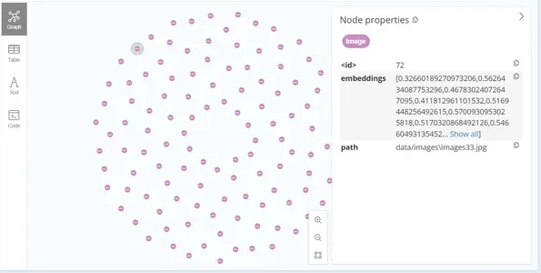
After the data insertion, the graph looks like this:

Part 2: Image Retrieval

For the inference part, where we need to predict the similar images, we will be using the cosine similarity metric. Cosine similarity is a measure of similarity between two non-zero vectors of an inner product space. It is defined to equal the cosine of the angle between them, which is also the same as the inner product of the same vectors normalized to both have length 1. We will be using the embeddings generated by the ResNet50 model to calculate the cosine similarity between the query image and the images in the database. The images with the highest cosine similarity will be the most similar to the query image.

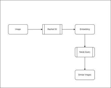
First the image embeddings are generated for the query image. Then it is passed to the Neo4j database to retrieve the similar images.

MATCH (a:Image)
WITH a, gds.similarity.cosine(a.embeddings, $query_embeddings) AS similarity
ORDER BY similarity DESC
LIMIT $top_k
RETURN a.id AS image_id, a.embeddings AS embeddings, a.path as image_path, similarity

The above query returns the top k similar images to the query image. The query returns the image id, image path, and the cosine similarity between the query image and the retrieved images. Use the cosine similarity to rank the images in descending order. Return the top k images. The node also have the image path as a property, which can retrieve the image from the file system.

The Neo4j server performs these computations, resulting in significantly faster processing compared to client-side execution. This efficiency is attributed to the server’s optimization for graph computations. Node properties store the embeddings in a columnar format, facilitating rapid retrieval. Additionally, the Neo4j server handles the computation of cosine similarity, leveraging its optimization for graph computations. This allows for faster retrieval of similar images.

Streamlit App

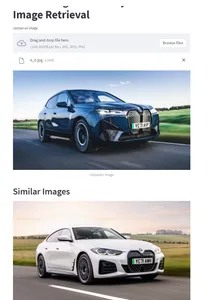
I have created a sample StreamLit app to test our logics.

The UI have an option to upload an image. It processes in the below flow get fetch the relevant images.

•  Generates Image embeddings using Resnet50 model
• Queries Neo4j DB to fetch similar embeddings and image locations
• Displays the similar images back to the UI

Sounds interesting?

The code for the sample app is here.

Creating Relations Between Nodes

Let’s say, if we are handling with only limited images and we want to create relations between them. We can use the following code to create relations between the images.

This allows to avoid the similarity calculations for every query we do.

MATCH (n1:Image), (n2:Image)
WHERE id(n1) < id(n2)  // To avoid duplicate pairs and self-comparisons
WITH n1, n2, gds.similarity.cosine(n1.embeddings, n2.embeddings) AS similarity
WHERE similarity > 0.8
CREATE (n1)-[:SIMILAR_TO {score: similarity}]->(n2)

This creates a relations, and it can be visible in the Neo4j graph.

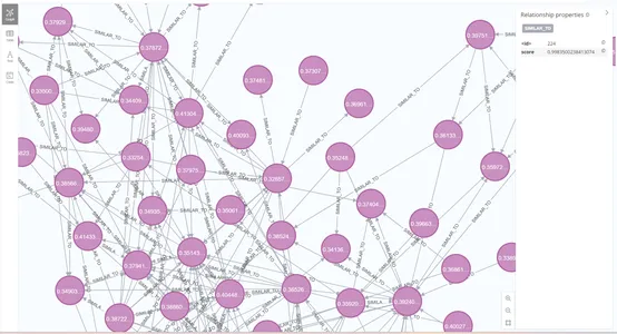
When we query the database for similar images, we can also include the relations in the query. This will allow us to retrieve the similar images along with the relations between them. Use this  to visualize the relations between the images.

MATCH (a:Image)-[r:SIMILAR_TO]->(b:Image)
WITH a, b, gds.similarity.cosine(a.embeddings, $query_embeddings) AS similarity, r
ORDER BY similarity DESC
LIMIT $top_k
RETURN a.id AS image_id, a.embeddings AS embeddings, a.path as image_path, similarity, r

Conclusion

In this article, we saw how to generate embeddings for images using a pre-trained model. We also saw how to store the embeddings and image paths in Neo4j. Finally, we saw how to retrieve similar images using the cosine similarity metric. This approach enables efficient retrieval of similar images. It finds applications in various domains, including e-commerce, content sharing platforms, healthcare, and more. Based on the data set we have, we can also try different image embeddings models and similarity metrics to play around.

Frequently Asked Questions

The media shown in this article is not owned by Analytics Vidhya and is used at the Author’s discretion.