What is Adam Optimizer?

In deep learning, optimization algorithms are essential for efficient learning and convergence in neural networks. One of the most popular choices is the Adam optimizer. So, what is the Adam optimizer? This blog post explores its inner workings, advantages, and practical tips for effective use.

This article was published as a part of the Data Science Blogathon.

What is Adam Optimizer?

The Adam optimizer, short for “Adaptive Moment Estimation,” is an iterative optimization algorithm used to minimize the loss function during the training of neural networks. Adam can be looked at as a combination of RMSprop and Stochastic Gradient Descent with momentum. Developed by Diederik P. Kingma and Jimmy Ba in 2014, Adam has become a go-to choice for many machine learning practitioners.

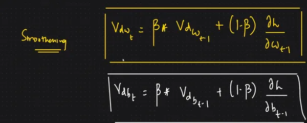
It uses the squared gradients to scale the learning rate like RMSprop, and it takes advantage of momentum by using the moving average of the gradient instead of the gradient itself, like SGD with momentum. This combines Dynamic Learning Rate and Smoothening to reach the global minima.

How Adam Optimizer Works?

By doing all of this, Adam helps the neural network learn more efficiently and effectively. It’s like having a good coach who guides the network to become better at its task.

What is Adam Optimization Algorithm?

Where w is model weights, b is for bias, and eta (looks like the letter n) is the step size (it can depend on iteration). And that’s it, that’s the update rule for Adam, which is also known as the Learning rate.

Steps Involved in the Adam Optimization Algorithm

• Initialize the first and second moments’ moving averages (m and v) to zero.
• Compute the gradient of the loss function to the model parameters.
• Update the moving averages using exponentially decaying averages. This involves calculating m_t and v_t as weighted averages of the previous moments and the current gradient.
• Apply bias correction to the moving averages, particularly during the early iterations.
• Calculate the parameter update by dividing the bias-corrected first moment by the square root of the bias-corrected second moment, with an added small constant (epsilon) for numerical stability.
• Update the model parameters using the calculated updates.
• Repeat steps 2-6 for a specified number of iterations or until convergence.

Key Features of Adam Optimizer

Adaptive Learning Rates

Adam adjusts the learning rates for each parameter individually. It calculates a moving average of the first-order moments (the mean of gradients) and the second-order moments (the uncentered variance of gradients) to scale the learning rates adaptively. This makes it well-suited for problems with sparse gradients or noisy data.

Bias Correction

To counteract the initialization bias in the first moments, Adam applies bias correction during the early iterations of training. This ensures faster convergence and stabilizes the training process.

Low Memory Requirements

Unlike some optimization algorithms that require storing a history of gradients for each parameter, Adam only needs to maintain two moving averages per parameter. This makes it memory-efficient, especially for large neural networks.

Practical Tips for using Adam Optimizer

• Learning Rate: While Adam adapts the learning rates, choosing a reasonable initial learning rate is still essential. It often performs well with the default value of 0.001.
• Epsilon Value: The epsilon (ε) value is a small constant added for numerical stability. Typical values are in the range of 1e-7 to 1e-8. It’s rarely necessary to change this value.
• Monitoring: Monitor your training process by monitoring the loss curve and other relevant metrics. Adjust learning rates or other hyperparameters if necessary.
• Regularization: Combine Adam with regularization techniques like dropout or weight decay to prevent overfitting.

Adam Optimizer Example with Code

Gradient Descent With Adam

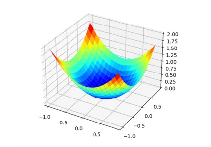
First, let’s define an optimization function. We will use a simple two-dimensional function that squares the input of each dimension and defines the range of valid inputs from -1.0 to 1.0.

The objective() function below implements this function.

from numpy import arange
from numpy import meshgrid
from matplotlib import pyplot

def objective(x, y):
    return x**2.0 + y**2.0

# define range for input
range_min, range_max = -1.0, 1.0

# sample input range uniformly at 0.1 increments
xaxis = arange(range_min, range_max, 0.1)
yaxis = arange(range_min, range_max, 0.1)

# create a mesh from the axis
x, y = meshgrid(xaxis, yaxis)

results = objective(x, y)

figure = pyplot.figure()
axis = figure.add_subplot(111, projection='3d')  
axis.plot_surface(x, y, results, cmap='jet')

# show the plot
pyplot.show()

Adam in Neural Network

Here’s a simplified Python code example demonstrating how to use the Adam optimizer in a neural network training scenario using the popular deep learning library TensorFlow. In this example, we’ll use TensorFlow’s Keras API for creating and training a simple neural network for image classification:

Importing Library

import keras # Import the Keras library
from keras.datasets import mnist # Load the MNIST dataset
from keras.models import Sequential # Initialize a sequential model
from keras.layers import Dense, Dropout, Flatten
from keras.layers import Conv2D, MaxPooling2D
import numpy as np

Split Data in Train and Test

# Load the MNIST dataset from Keras
(x_train, y_train), (x_test, y_test) = mnist.load_data()

# Print the shape of the training and test data
print(x_train.shape, y_train.shape)

# Reshape the training and test data to 4 dimensions
x_train = x_train.reshape(x_train.shape[0], 28, 28, 1)

x_test = x_test.reshape(x_test.shape[0], 28, 28, 1)

# Define the input shape
input_shape = (28, 28, 1)

# Convert the labels to categorical format
y_train = keras.utils.to_categorical(y_train)
y_test = keras.utils.to_categorical(y_test)

# Convert the pixel values to floats between 0 and 1
x_train = x_train.astype('float32')
x_test = x_test.astype('float32')

# Normalize the pixel values by dividing them by 255
x_train /= 255
x_test /= 255

# Define the batch size and number of classes
batch_size = 60
num_classes = 10

# Define the number of epochs to train the model for
epochs = 10

Define Model Function

"""
  Builds a CNN model for MNIST digit classification.

  Args:
    optimizer: The optimizer to use for training the model.

  Returns:
    A compiled Keras model.
  """

def build_model(optimizer):
    model = Sequential()
    model.add(Conv2D(32, kernel_size=(3, 3), activation='relu', input_shape=input_shape))
    model.add(MaxPooling2D(pool_size=(2, 2)))
    model.add(Dropout(0.25))
    model.add(Flatten())
    model.add(Dense(128, activation='relu'))
    model.add(Dropout(0.5))
    model.add(Dense(num_classes, activation='softmax'))
    model.compile(loss='categorical_crossentropy', optimizer=optimizer, metrics=['accuracy'])
    return model

Optimization in Neural Network

optimizers=['Adagrad','Adam','SGD']#import csv
histories ={opt:build_model(opt).fit(x_train,y_train,batch_size=batch_size, 
epochs=epochs,verbose=1,validation_data=(x_test,y_test)) for opt in optimiers}

Advantages of using Adam Optimizer

• Fast Convergence: Adam often converges faster than traditional gradient descent-based optimizers, especially on complex loss surfaces.
• Adaptive Learning Rates: The adaptive learning rates make it suitable for various machine learning tasks, including natural language processing, computer vision, and reinforcement learning.
• Low Memory Usage: Low memory requirements allow training large neural networks without running into memory constraints.
• Robustness: Adam is relatively robust to hyperparameter choices, making it a good choice for practitioners without extensive hyperparameter tuning experience.

Common Challenges with Adam Optimizer

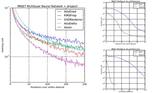
ADAM paper presented diagrams that showed even better results:

Recent research has raised concerns about the generalization capabilities of the Adam optimizer in deep learning, indicating that it may not always converge to optimal solutions, particularly in tasks like image classification on CIFAR datasets. Wilson et al.’s study highlighted that adaptive optimizers like Adam might not generalize as effectively as SGD with momentum across various deep-learning tasks.

Nitish Shirish Keskar and Richard Socher proposed a solution called SWATS, where training begins with Adam but switches to SGD as learning saturates. SWATS has shown promise in achieving competitive generalization performance compared to SGD with momentum, prompting a reevaluation of optimization choices in deep learning.

Conclusion

Adam is one of the best optimization algorithms for deep learning, and its popularity is growing quickly. Its adaptive learning rates, efficiency in optimization, and robustness make it a popular choice for training neural networks. As deep learning evolves, optimization algorithms like Adam optimizer will remain essential tools. Still, practitioners should stay open to alternative approaches and strategies for achieving optimal model performance.

I want to take a moment to say thank you. Thank you for taking the time to read this blog and for your interest in Adam Optimizer in Neural Networks.

Until next time, stay curious and keep learning!

Frequently Asked Questions

The media shown in this article is not owned by Analytics Vidhya and is used at the Author’s discretion.

Neha Vishwakarma

I'm Neha Vishwakarma, a data science enthusiast with a background in information technology, dedicated to using data to inform decisions and tackle complex challenges. My passion lies in uncovering hidden insights through numbers.