Introduction
In natural language processing (NLP), it is important to understand and effectively process sequential data. Long Short-Term Memory (LSTM) models have emerged as a powerful tool for tackling this challenge. They offer the capability to capture both short-term nuances and long-term dependencies within sequences. Before delving into the intricacies of LSTM language translation models, it’s crucial to grasp the fundamental concept of LSTMs and their role within Recurrent Neural Networks (RNNs). This article provides a comprehensive guide to understanding, implementing, and evaluating LSTM models for language translation tasks, with a focus on translating English sentences into Hindi. Through a step-by-step approach, we will explore the architecture, preprocessing techniques, model building, training, and evaluation of LSTM models.

Learning Objective
- Understand the fundamentals of LSTM architecture.
- Learn how to preprocess sequential data for LSTM models.
- Implement LSTM models for sequence prediction tasks.
- Evaluate and interpret LSTM model performance.
Table of Contents
- What is RNN?
- What is LSTM?
- Problem Statement
- Step 1: Loading the Data from Hugging Face
- Step 2: Importing Necessary Libraries
- Step 3: Data Preprocessing
- Step 4: Tokenization and Sequence Padding
- Step 5: Splitting Data into Training and Validation Sets
- Step 6: Building The LSTM Model
- Step 7: Compiling and Training the Model
- Step 8: Plotting Training and Validation Loss
- Frequently Asked Questions
What is RNN?
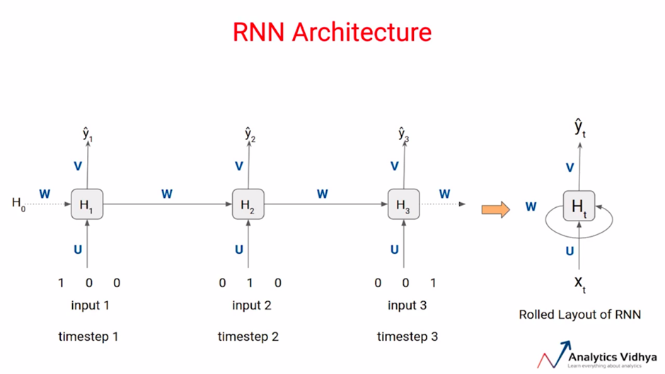
Recurrent Neural Networks (RNNs) serve a crucial purpose in the area of neural networks due to their unique ability to handle sequential data effectively. Unlike other types of neural networks, RNNs are specifically designed to capture dependencies within sequential data points.
Consider the example of text data, where each data point Xi represents a sequence of words or sentences. In natural language, the order of words matters significantly, as well as the semantic relationships between them. However, conventional neural networks often overlook this aspect, treating the input as an unordered set of features. Consequently, they struggle to comprehend the inherent structure and meaning within the text.
RNNs address this limitation by maintaining relationships between words across the entire sequence. They achieve this by introducing a time axis, essentially creating a looped structure where each word in the input sequence is processed sequentially, incorporating information from both the current word and the context provided by previous words.
This structure allows RNNs to capture short-term dependencies within the data. However, they still face challenges in preserving long-term dependencies effectively. In the context of the time axis illustration, RNNs encounter difficulty in maintaining strong connections between the first and last words of the sequence. This is primarily due to the tendency for earlier inputs to have less influence on later predictions, leading to the potential loss of context and meaning over longer sequences.
What is LSTM?
Before delving into LSTM language translation models, it’s essential to grasp the concept of LSTMs.
LSTM stands for Long Short-Term Memory, which is a specialized type of RNN. As the name suggests, LSTMs are designed to effectively capture both long-term and short-term dependencies within sequential data. If you’re interested in learning more about RNNs and LSTMs, you can explore the resources available here and here. But let me provide you with a concise overview of them.
LSTMs gained popularity for their ability to address the limitations of traditional RNNs, particularly in maintaining both long-term and short-term dependencies within sequential data. This achievement is facilitated by the unique structure of LSTMs.
The LSTM structure may initially appear intricate, but I’ll simplify it for better understanding. The time axis of a data point, labeled as xt0 to xtn, corresponds to individual blocks representing cell states, denoted as h_t, which output the corresponding cell state. The yellow square boxes represent activation functions, while the round pink boxes signify pointwise operations. Let’s delve into the core concept.
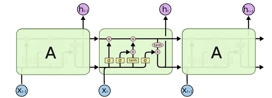
The fundamental idea behind LSTMs is to manage long-term and short-term dependencies effectively. This is accomplished by selectively discarding unimportant elements x_t while retaining critical ones through identity mapping. LSTMs can be distilled into three primary gates, each serving a distinct purpose.
1. Forget Gate
The Forget Gate determines the relevance of information from the previous state to be retained or discarded for the next state. It merges information from the previous hidden state h_t-1 and the current input x_t, passing it through a sigmoid function to produce values between 0 and 1. Values closer to 0 signify information to forget, while those closer to 1 indicate information to keep, achieved through appropriate weight backpropagation during training.
2. Input Gate
The Input Gate manages data updates to the cell state. It merges and processes the previous hidden state h_t-1 and the current input x_t through a sigmoid function, producing values between 0 and 1. These values, indicating importance, are pointwise multiplied with the output of the tanh function, which squashes values between -1 and 1 to regulate the network. The resulting product determines the relevant information to be added to the cell state.
3. Cell State
The Cell State combines the significant information retained from the Forget Gate (representing the important information from the previous state) and the Input Gate (representing the important information from the current state) through pointwise addition. This update yields a new cell state c_t that the neural network deems relevant.
4. Output Gate
Lastly, the Output Gate determines the information relevant to the next hidden state. It merges the previous hidden state and the current input into a sigmoid function to determine which information to retain. Simultaneously, the modified cell state is passed through a tanh function. The outputs are then multiplied to decide the information to carry forward to the next hidden state.
It’s important to note that the hidden state retains information from previous input states, making it useful for predictions, and is passed as the output for the current state h_t.
Problem Statement
Our aim is to utilize an LSTM sequence-to-sequence model to translate English sentences into their corresponding Hindi counterparts.
For this, I am taking a dataset from hugging face
Step 1: Loading the Data from Hugging Face
!pip install datasets
from datasets import load_dataset

df=load_dataset("Aarif1430/english-to-hindi")
df['train'][0]
import pandas as pd
da = pd.DataFrame(df['train'])  # Assuming you want to load the train split
da.rename(columns={'english_sentence': 'english', 'hindi_sentence': 'hindi'}, inplace=True)

da.head()
In this code, we install the dataset library if not already installed. Then, use the load_dataset function to load the English-Hindi dataset from Hugging Face. We convert the dataset into pandas DataFrame for further processing and display the first few rows to verify the data loading.
Step 2: Importing Necessary Libraries
import numpy as np
import string
from numpy import array, argmax, random, take
import pandas as pd
from keras.models import Sequential
from keras.layers import Dense, LSTM, Embedding, RepeatVector
from keras.preprocessing.text import Tokenizer
from keras.callbacks import ModelCheckpoint
from keras.preprocessing.sequence import pad_sequences
from keras.models import load_model
from keras import optimizers
from tensorflow.keras.models import Sequential
from tensorflow.keras.layers import Embedding, LSTM
import matplotlib.pyplot as plt
import tensorflow as tf
import warnings
warnings.filterwarnings("ignore")
Here, we have imported all the necessary libraries and modules required for data preprocessing, model building, and evaluation.
Step 3: Data Preprocessing
#Removing punctuations and converting text to lowercase for both languages
da['english'] = da['english'].str.replace('[{}]'.format(string.punctuation), '').str.lower()
da['hindi'] = da['hindi'].str.replace('[{}]'.format(string.punctuation), '').str.lower()

# Find indices of empty rows in both languages
eng_empty_indices = da[da['english'].str.strip().astype(bool) == False].index
hin_empty_indices = da[da['hindi'].str.strip().astype(bool) == False].index

# Combine indices from both languages to remove empty rows
remove_indices = list(set(eng_empty_indices) | set(hin_empty_indices))

# Removing empty rows
da.drop(remove_indices, inplace=True)

# Reset indices
da.reset_index(drop=True, inplace=True)
Here , we preprocess the data by removing punctuation and converting text to lowercase for both English and Hindi sentences. Additionally, we handle empty rows by finding and removing them from the dataset.
Step 4: Tokenization and Sequence Padding
# Importing necessary libraries
from tensorflow.keras.preprocessing.text import Tokenizer
from tensorflow.keras.preprocessing.sequence import pad_sequences

# Initialize Tokenizer for English subtitles
tokenizer_eng = Tokenizer()
tokenizer_eng.fit_on_texts(da['english'])

# Convert text to sequences of integers for English subtitles
sequences_eng = tokenizer_eng.texts_to_sequences(da['english'])

# Initialize Tokenizer for Hindi subtitles
tokenizer_hin = Tokenizer()
tokenizer_hin.fit_on_texts(da['hindi'])

# Convert text to sequences of integers for Hindi subtitles
sequences_hin = tokenizer_hin.texts_to_sequences(da['hindi'])

# Pad sequences to ensure uniform length
max_length = 100  # Define the maximum sequence length
sequences_eng = pad_sequences(sequences_eng, maxlen=max_length, padding='post')
sequences_hin = pad_sequences(sequences_hin, maxlen=max_length, padding='post')

# Verify the vocabulary sizes
vocab_size_eng = len(tokenizer_eng.word_index) + 1
vocab_size_hin = len(tokenizer_hin.word_index) + 1

print("Vocabulary size for English subtitles:", vocab_size_eng)
print("Vocabulary size for Hindi subtitles:", vocab_size_hin)
Here, we import the necessary libraries for tokenization and sequence padding. Then, we tokenize the text data for both English and Hindi sentences and convert them into sequences of integers. We pad the sequences to ensure uniform length, and finally, we print the vocabulary sizes for both languages.
Determining Sequence Lengths
eng_length = sequences_eng.shape[1]  # Length of English sequences
hin_length = sequences_hin.shape[1]  # Length of Hindi sequences
print(eng_length, hin_length)
In this, we are determining the lengths of the sequences for both English and Hindi sentences. The length of a sequence refers to the number of tokens or words in the sequence.
Step 5: Splitting Data into Training and Validation Sets
from sklearn.model_selection import train_test_split

# Split the training data into training and validation sets
X_train, X_val, y_train, y_val = train_test_split(sequences_eng[:50000], sequences_hin[:50000], test_size=0.2, random_state=42)

# Verify the shapes of the datasets
print("Shape of X_train:", X_train.shape)
print("Shape of y_train:", y_train.shape)
print("Shape of X_val:", X_val.shape)
print("Shape of y_val:", y_val.shape)
In this step, we are splitting the preprocessed data into training and validation sets.
Step 6: Building The LSTM Model
from keras.models import Sequential
from keras.layers import Dense, LSTM, Embedding, RepeatVector

model = Sequential()
model.add(Embedding(input_dim=vocab_size_eng, output_dim=128,input_shape=(eng_length,), mask_zero=True))
model.add(LSTM(units=512))
model.add(RepeatVector(n=hin_length))
model.add(LSTM(units=512, return_sequences=True))
model.add(Dense(units=vocab_size_hin, activation='softmax'))
This step involves building the LSTM sequence-to-sequence model for English to Hindi translation. Let’s break down the layers added to the model:
The first layer is an embedding layer (Embedding) which maps each word index to a dense vector representation. It takes as input the vocabulary size for English (vocab_size_eng), the output dimensionality (output_dim=128), and the input shape specified by the maximum sequence length for English (input_shape=(eng_length,)). Additionally, mask_zero=True is set to ignore padded zeros.
Next, we add an LSTM layer (LSTM) with 512 units, which processes the embedded sequences.
The RepeatVector layer repeats the output of the LSTM layer for hin_length times, preparing it to be fed into the subsequent LSTM layer.
Then, we add another LSTM layer with 512 units, set to return sequences (return_sequences=True), which is crucial for sequence-to-sequence models.
Finally, we add a dense layer (Dense) with a softmax activation function to predict the probability distribution over the Hindi vocabulary for each time step.
Printing the Model Summary
model.summary()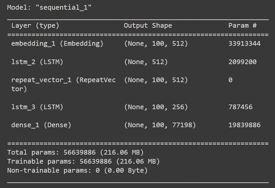
Step 7: Compiling and Training the Model
from tensorflow.keras.optimizers import RMSprop

# Define optimizer
rms = RMSprop(learning_rate=0.001)

# Compile the model
model.compile(optimizer=rms, loss='sparse_categorical_crossentropy', metrics=['accuracy'])

# Train the model
history = model.fit(X_train, y_train, validation_data=(X_val, y_val), epochs=10, batch_size=32)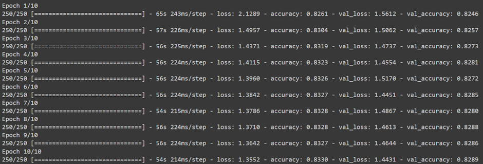
This step compiles the LSTM model with rms optimizer, sparse_categorical_crossentropy loss function, and accuracy metrics. Then, it trains the model on the provided data for 10 epochs, using a batch size of 32. The training process yields a history object capturing training metrics over epochs.
Step 8: Plotting Training and Validation Loss
import matplotlib.pyplot as plt

# Get the training history
loss = history.history['loss']
val_loss = history.history['val_loss']
epochs = range(1, len(loss) + 1)

# Plot loss and validation loss with custom colors
plt.plot(epochs, loss, 'r', label='Training Loss')  # Red color for training loss
plt.plot(epochs, val_loss, 'g', label='Validation Loss')  # Green color for validation loss
plt.title('Training and Validation Loss')
plt.xlabel('Epochs')
plt.ylabel('Loss')
plt.legend()
plt.show()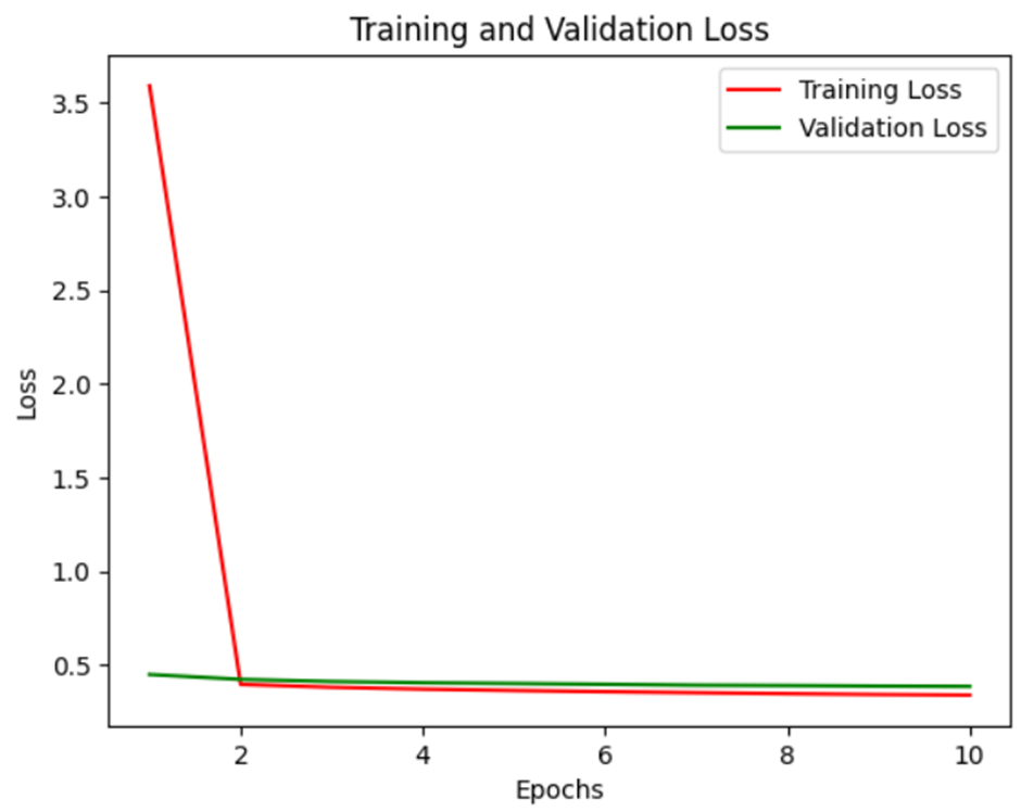
This step involves plotting the training and validation loss over epochs to visualize the model’s learning progress and potential overfitting.
Conclusion
This guide navigates the creation of an LSTM sequence-to-sequence model for English-to-Hindi language translation. It begins with an overview of RNNs and LSTMs, emphasizing their ability to handle sequential data effectively. The objective is to translate English sentences into Hindi using this model.
Steps include data loading from Hugging Face, preprocessing to remove punctuation and handle empty rows, and tokenization with sequence padding for uniform length. The LSTM model is meticulously built with embedding, LSTM, RepeatVector, and dense layers. Training involves compiling the model with an optimizer, loss function, and metrics, followed by fitting it to the dataset over epochs.
Visualizing training and validation loss offers insights into the model’s learning progress. Ultimately, this guide empowers users with the skills to construct LSTM models for language translation tasks, providing a foundation for further exploration in NLP.
Frequently Asked Questions
A. An LSTM (Long Short-Term Memory) sequence-to-sequence model is a type of neural network architecture designed to translate sequences of data from one language to another. It utilizes LSTM units to capture both short-term and long-term dependencies within sequential data effectively.
A. The LSTM model processes input sequences, typically in English, and generates corresponding output sequences, usually in another language like Hindi. It does so by learning to encode the input sequence into a fixed-size vector representation and then decoding this representation into the output sequence.
A. Preprocessing steps include removing punctuation, handling empty rows, tokenizing the text into sequences of integers, and padding the sequences to ensure uniform length.
A. Common evaluation metrics include training and validation loss, which measure the discrepancy between predicted and actual sequences during training. Additionally, metrics like BLEU score can be used to evaluate the model’s performance.
A. Performance can be improved by experimenting with different model architectures, adjusting hyperparameters such as learning rate and batch size, increasing the size of the training dataset, and employing techniques like attention mechanisms to focus on relevant parts of the input sequence during translation.
A. Yes, the LSTM model can be adapted to translate between pairs of languages other than English and Hindi. By training the model on datasets containing sequences in different languages, it can learn to perform translation tasks for those language pairs as well.


