Is Jasprit Bumrah a Genius Bowler? Using AutoEncoders for Anomaly Detection in Cricket

Introduction

During one of the cricket matches in the ICC World Cup T20 Championship, Rohit Sharma, Captain of Indian Cricket Team had applauded Jasprit Bumrah as Genius Bowler. I decided to run a experiment and test it out using data available publicly. Even though it is a fun project, I was pleasantly surprised by the results. Let us get started.

Problem Definition

To do data analysis or building models, we need to convert business problem into data problem. How do we make our model understand meaning of Genius. Well, Genius can be defined as “Way over or Head and Shoulders above the rest”. Can we formulate this as an Anomaly detection problem? Yes.

There are many ways to solve Anomaly detection problem. We would stick to AutoEncoders using PyTorch.

We would use publicly available T20 Player Statistics from cricket data R package to train our AutoEncoders model. If AutoEncoders struggles to reconstruct values then Mean Square Error (MSE) would be high. MSE over a threshold would be an anomaly.

In our case, MSE for Jasprit Bumrah should be sufficiently high to be flagged as anomaly or Genius.

Learning Objectives

• Grasp the basic architecture of AutoEncoders, including the roles of the encoder and decoder networks.
• Understand how to utilize reconstruction error (Mean Squared Error) from AutoEncoders to identify anomalies.
• Learn to preprocess data, create datasets, and set up data loaders for training and testing models.
• Understand the process of training an AutoEncoders, including setting hyperparameters, loss functions, and optimizers.
• Explore real-world applications of anomaly detection, such as customer management and fraud detection.

This article was published as a part of the Data Science Blogathon.

What are AutoEncoders?

AutoEncoders are composed of two networks Encoder and Decoder. Encoder receives D dimensional vector V and encodes into a vector X of M dimension wherein M < D. Hence, Encoder compresses our Input. Decoder decompresses X and tries to recreate V as far as possible. Let us call output of Decoder as Z.

Typically, Decoder would able to recreate V for most of rows i.e for most rows Z would be closer to V. But for certain rows, Decoder would struggle to decode and difference between Z and V would be huge. We would call these values Anomaly. Anomaly values usually have high Mean Squared Error or MSE.

Real World Applications of AutoEncoder

Let us now explore real world applications of AutoEncoder.

Customer Management

Suppose a Organization deals with lot of customers and has a methodology to label Customers as good or bad, clean or risky, wealthy or non wealthly. Auto Encoder when trained only on good or clean or wealthly customers can decipher pattern on these top or ideal customers. When a new customer comes in we have a reliable way to know how different is the new customer from ideal customer. You may argue that it can be done manually. Humans are limited by amount of variables and data they can handle. Machines do not have this limitation.

Fraud Management

Similar to above, if a organization has methodology to label transactions as fraudulent or non fraudulent. We can train our Autoencoder on Non-Fradulent transactions alone and in production environments, we have a reliable mechanism to know how different the new transaction from ideal transaction.

Above is not exhaustive list of application of AutoEncoder.

Let us now go back to our original problem.

Data Collection, Cleaning and Feature Engineering

 I collected T20 career statistics data of bowlers here.

I used R library cricketdata to download player T20 Career Statistics as python version of the same is not available as far as i know. T20 Statistics does not include leagues like IPL.

library(cricketdata)
# T20 Career Data
t20_career <- fetch_cricinfo("T20", "men", "Bowling",'career')
# T20 Innings Data
t20_innings <- fetch_cricinfo("T20", "men", "Bowling",'innings')

We need to join both these datasets and create final input dataset to be used for training AutoEncoders in Python. Before saving the file to disk we need to consider only Test Playing Countries for our Analysis.

final<-final[Country %in% c('Australia','West Indies','South Africa'
                            ,'Pakistan','Afghanistan','India'
                            ,'Sri Lanka','England','New Zealand'
                            ,'BAN')]
fwrite(final,'T20_Stats_Career.txt',sep="|")

We can name the final dataset as “T20_Stats_Career.txt”.

Now we will use Python for our rest of Analysis.

import numpy as np
import torch
import torch.optim as optim
import numpy as np
import torch
import torch.optim as optim
import torch.nn as nn
from torch.utils.data import TensorDataset,DataLoader
from sklearn.preprocessing import StandardScaler
import pandas as pd
import matplotlib.pyplot as plt
import seaborn as sns
import random

We have imported all necessary libraries. We would now read Player’s data.

df = pd.read_csv('T20_Stats_Career.txt',sep='|')
df.head()

For every player, we have data of Number of Innings, Overs, Maidens, Runs, Wickets, Average, Economy and Strike Rate.

Feature Engineering

I have added two new features:

• Maiden Percentage: No of Maidens / No of Overs
• Wickets Per Over:  No of Wickets / No of Overs

df['Maiden_PCT'] = df['Maidens'] / df['Overs'] * 100
df['Wickets_Per_over'] = df['Wickets'] / df['Overs']

We also need to drop Players with Number of Innings less than 15 so that we use only those players with sufficient match experience for our Analysis.

Train and Test Dataset

 Train Dataset: Train Datasets would have T20 Statistics of players from nationalities other than India.

Test Dataset: Only Indian Players.

# Create Train and Test Dataset
test = df[df['Country'] == 'India']
train = df[df['Country'] != 'India']

We use the following features to train our Model:

• Average
• Economy
• Strike Rate
• No of Four Wickets
• No of Five Wickets
• Maiden Percentage
• Wickets Per Over

Drop Unnecessary Features

features = ['Average','Economy','StrikeRate','FourWickets','FiveWickets'
,'Maiden_PCT','Wickets_Per_over']
X_train = train[features]
X_test = test[features]
print("Number of Players in Train Dataset",X_train.shape)
print("Number of Players in Test Dataset",X_test.shape)
X_train.head()

Data Standarization

We have train and test dataset. Now we need to standardize the data.

sc = StandardScaler()
sc.fit(X_train)
X_train = sc.transform(X_train)
X_test = sc.transform(X_test)

Model Training

We now set appropriate device and set data loaders with batch size of 16.

# Create Tensor Dataset and Dataloders
device = 'cuda' if torch.cuda.is_available() else 'cpu'

torch.manual_seed(13)
x_train_tensor = torch.as_tensor(X_train).float().to(device)
y_train_tensor = torch.as_tensor(X_train).float().to(device)

x_test_tensor = torch.as_tensor(X_test).float().to(device)
y_test_tensor = torch.as_tensor(X_test).float().to(device)

train_dataset = TensorDataset(x_train_tensor,y_train_tensor)
test_dataset = TensorDataset(x_test_tensor,y_test_tensor)

train_loader = DataLoader(dataset=train_dataset,batch_size=16,shuffle=True)
test_loader = DataLoader(dataset=test_dataset,batch_size=16)

We set AutoEncoders Architecture as below:

7 ->4->2->4->7.

As we are dealing with very less data we would build a simple model.

We use Learning Rate as 0.001 and Adam as Optimizer.

# AutoEncoder Architecture

class AutoEncoder(nn.Module):
    def __init__(self):
        super(AutoEncoder,self).__init__()
        self.encoder = nn.Sequential()
        self.encoder.add_module('Hidden1',nn.Linear(7,4))
        self.encoder.add_module('Relu1',nn.ReLU())
        self.encoder.add_module('Hidden2',nn.Linear(4,2))
        
        self.decoder = nn.Sequential()
        self.decoder.add_module('Hidden3',nn.Linear(2,4))
        self.decoder.add_module('Relu2',nn.ReLU())
        self.decoder.add_module('Hidden4',nn.Linear(4,7))

    def forward(self,x):
        encoder = self.encoder(x)
        return self.decoder(encoder)
        
    # Predict Method
    def predict(model,x):

        model.eval()
        x_tensor = torch.as_tensor(x).float()
        y_hat = model(x_tensor.to(device))
        model.train()

        return y_hat.detach().cpu().numpy()

    # Plot Losses
     def plot_losses(train_losses,test_losses):
        fig = plt.figure(figsize=(10,4))
        plt.plot(train_losses,label='training_loss',c='b')
        #plt.plot(self.val_losses,label='val loss',c='r')
        if test_loader:
            plt.plot(test_losses,label='test loss',c='r')
        #plt.yscale('log')
        plt.xlabel('Epochs')
        plt.ylabel('Loss')
        plt.legend()
        plt.tight_layout()
        return fig

# Model Loss and Optimizer
lr = 0.001
torch.manual_seed(21)
model = AutoEncoder().to(device)
optimizer = optim.Adam(model.parameters(),lr = lr)
loss_fn =nn.MSELoss()

We train our model for 250 epochs.

num_epochs=250
train_loss=[]
test_loss=[]
seed=42
torch.backends.cudnn.deterministic=True
torch.backends.cudnn.benchmark=False
torch.manual_seed(seed)
np.random.seed(seed)
random.seed(seed)
for epoch in range(num_epochs):
    mini_batch_train_loss=[]
    mini_batch_test_loss=[]
    for train_batch,y_train in train_loader:
        train_batch =train_batch.to(device)
        model.train()
        yhat = model(train_batch)
        loss = loss_fn(yhat,y_train)
        mini_batch_train_loss.append(loss.cpu().detach().numpy())
        
        loss.backward()
        optimizer.step()
        optimizer.zero_grad()
  
    train_epoch_loss = np.mean(mini_batch_train_loss)
    train_loss.append(train_epoch_loss)

    with torch.no_grad():
        for test_batch,y_test in test_loader:
            test_batch = test_batch.to(device)
            model.eval()
            yhat = model(test_batch)
            loss = loss_fn(yhat,y_test)
            mini_batch_test_loss.append(loss.cpu().detach().numpy())
        test_epoch_loss = np.mean(mini_batch_test_loss)
        test_loss.append(test_epoch_loss)
        
fig = plot_losses(train_loss,test_loss)
fig.savefig('Train_Test_Loss.png')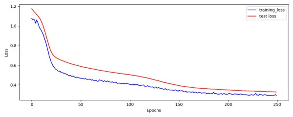

Train and Test Loss plot looks OK.

Mean Squared Error (MSE)

Using Predict Function we can predict for Train Dataset. We then compute Mean Squared Error by squaring difference between Actuals and Predicted. Also we will compute Z-Score using mean and standard deviation of MSE.

# Predict Train Dataset and get error
train_pred = predict(model,X_train)
print(train_pred.shape)
error = np.mean(np.power(X_train - train_pred,2),axis=1)
print(error.shape)
train['error'] = error
mean_error = np.mean(train['error'])
std_error =np.std(train['error'])
train['zscore'] = (train['error'] - mean_error) / std_error
train = train.sort_values(by='error').reset_index()
train.to_csv('Train_Output.txt',sep="|",index=None)

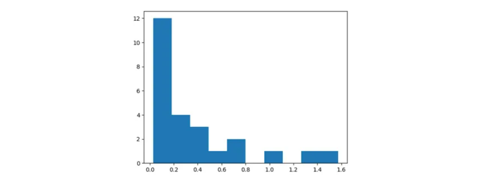
fig = plt.figure(figsize=(10,4))
plt.title('Distribution of MSE in Train Dataset')
train['error'].plot(kind='line')
plt.ylabel('MSE')
plt.show()
fig.savefig('Train_MSE.png')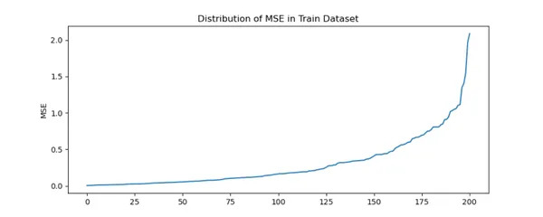

We can infer there is steep increase in MSE for certain players.

Majority of players are within MSE of 1. Beyond 1.2 MSE there are only few players.

Top 3 Players in the train dataset with highest MSE are:

train.tail(3)

Please keep in mind that we are using Tail Function

We can infer that for some players auto encoder struggles to reconstruct original values resulting in high MSE.

By looking at above plots, we can set threshold to be 1.2.

I agree that we need to split data into train and validation and use data of validation dataset to set threshold. But in this case we have only 200 rows. We are forced to take this approach.

Test Dataset – Indian Players or Bowlers

Let us now compute Mean Squared Error and ZScore for Test Data.

# Predict Test Dataset and get error
test_pred = predict(model,X_test)
test_error = np.mean(np.power(X_test - test_pred,2),axis=1)
test['error'] = test_error
test['zscore'] = (test['error'] - mean_error) / std_error
test = test.sort_values(by='error').reset_index()
test.to_csv('Test_Output.txt',sep="|",index=None)

fig = plt.figure(figsize=(10,4))
plt.title('Distribution of MSE in Test Dataset')
test['error'].plot(kind='line')
plt.ylabel('MSE')
plt.show()
fig.savefig('Test_MSE.png')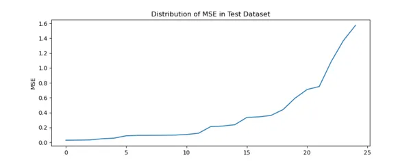

Similar to Train Dataset there is steep increase in MSE for certain Indian Players.

test.tail(3)

Please keep in mind that we are using Tail Function. Hence Correct order is Kuldeep Yadav, JJ Bumrah and Harbhajan Singh.

As in train dataset, we create a new column named Error in test dataset which has MSE values. Similar to Train Dataset, Autoencoder is struggling to reconstruct original values for some Indian Players.

Using Train MSE we have computed mean and standard deviation. For each value in test dataset we compute Z-Score as (test error – train mean error) / train error standard deviation.

We can verify that Z-Score for Bumrah is more than 3 which signifies Anomaly or Genius.

MSE Breakdown or Drill Down

Let us now learn about the MSE breakdown for the players.

Jasprit Bumrah

Let us now, understand why MSE is high for Jasprit Bumrah. MSE of Jasprit Bumrah is 1.36. Let us drill down further on the MSE at variable level to understand contributing factors.

MSE is calculated as (Actual – Predicted) * (Actual – Predicted).

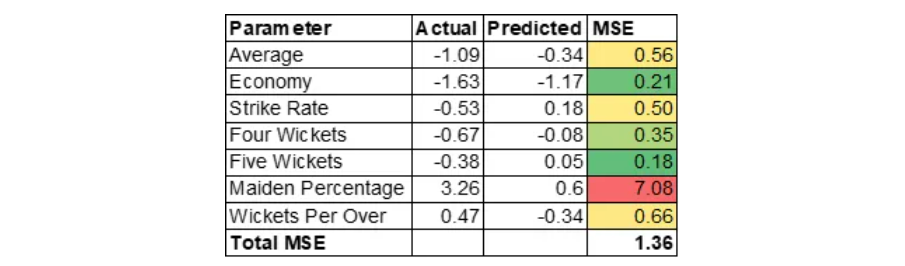
Please note that we are dealing with standardized values. Reason for the high MSE is mostly contributed by high Maiden Percentage. This means Bumrah would be an outstanding bowler at 19th or 20th over of the innings. High Maiden Percentage would create pressure on batsman which can result in other bowlers taking wickets in the next over. Please note that variable Maiden Percentage is was created by Feature Engineering.

Kuldeep Yadav

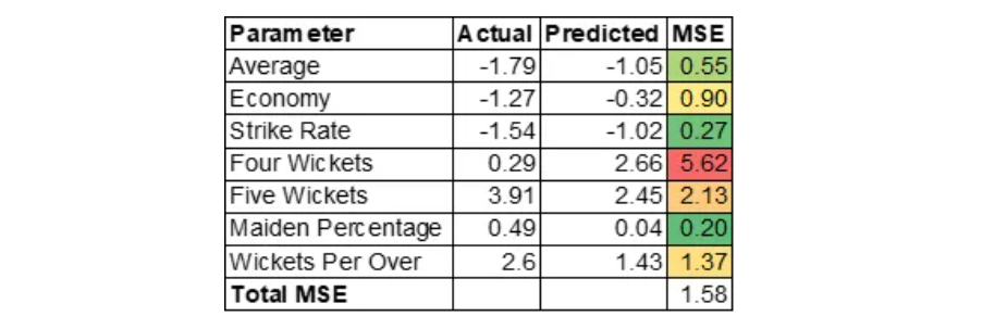
Kuldeep Yadav has uncanny ability of picking up wickets which will be useful in middle overs. Auto Encoder over predicted four wickets variable.

Overall Statistics of Top 2 Indian Bowlers

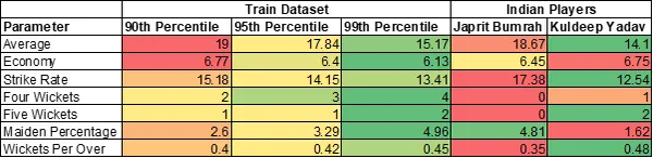
Jasprit Bumrah has 2 variables in more than 90th percentile. Kuldeep Yadav has 4 variables in more than 99th percentile.

Hope to see Kuldeep Yadav in action soon.

You can find full code here.

Conclusion

AutoEncoder is a powerful tool in one’s arsenal for Anomaly Detection but it is not the only method. We can also consider using ML algorithms like Isolation Forest or other simpler methods. Coming back to our problem, we can infer that AutoEncoder is able to correctly identify Anomalies. Toughest part in Anomaly Detection is to convince stakeholders of the reasons of the Anomaly. Here we computed drill down of MSE to identify reasons for the Anomaly. These insights are as important as detecting anomaly itself. Explainable AI is important.

Key Takeaways

• We used R Package cricketdata to download T20 Player Statistics for test playing nations and save the data to disk.
• Do Feature Engineering by computing Maiden Percentage and Wickets Per Over.
• Using PyTorch we would train Auto Encoder model for 250 epochs on the Train Dataset. We use optimizer as Adam and set learning rate to 0.001.
• Compute Mean Square Error by computing difference between Actual and Prediction in both train and test dataset.
• We consider Reconstruction error beyond a certain threshold as an anomaly. In our case it is 1.2.
• By looking at break up of MSE we can infer that Bumrah excels in bowling Maidens which is gold in T20.

Frequently Asked Questions

The media shown in this article is not owned by Analytics Vidhya and is used at the Author’s discretion.

Balajisr SR 26 Jun, 2024

Data Enthusiast. Love to bridge gap between data and strategy and work on anything in between which includes data science.