Introduction
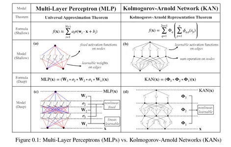
Kolmogorov-Arnold Networks, also known as KAN, are the latest advancement in neural networks. Based on the Kolgomorov-Arnold representation theorem, they have the potential to be a viable alternative to Multilayer Perceptrons (MLP). Unlike MLPs with fixed activation functions at each node, KANs use learnable activation functions on edges, replacing linear weights with univariate functions as parameterized splines.
A research team from the Massachusetts Institute of Technology, California Institute of Technology, Northeastern University, and The NSF Institute for Artificial Intelligence and Fundamental Interactions presented Kolmogorov-Arnold Networks (KANs) as a promising replacement for MLPs in a recent paper titled “KAN: Kolmogorov-Arnold Networks.”

Learning Objectives
- Learn and understand a new type of neural network called Kolmogorov-Arnold Network that can provide accuracy and interpretability.
- Implement Kolmogorov-Arnold Networks using Python libraries.
- Understand the differences between Multi-Layer Perceptrons and Kolmogorov-Arnold Networks.
This article was published as a part of the Data Science Blogathon.
Table of contents
Kolmogorov-Arnold representation theorem
According to the Kolmogorov-Arnold representation theorem, any multivariate continuous function can be defined as:
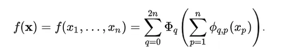
Here:
ϕqp : [0, 1] → R and Φq : R → R
Any multivariate function can be expressed as a sum of univariate functions and additions. This might make you think machine learning can become easier by learning high-dimensional functions through simple one-dimensional ones. However, since univariate functions can be non-smooth, this theorem was considered theoretical and impossible in practice. However, the researchers of KAN realized the potential of this theorem by expanding the function to greater than 2n+1 layers and for real-world, smooth functions.
What are Multi-layer Perceptrons?
These are the simplest forms of ANNs, where information flows in one direction, from input to output. The network architecture does not have cycles or loops. Multilayer perceptrons (MLP) are a type of feedforward neural network.
Multilayer Perceptrons are a type of feedforward neural network. Feedforward Neural Networks are simple artificial neural networks in which information moves forward, in one direction, from input to output via a hidden layer.
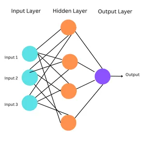
Working of MLPs
- Input Layer: The input layer consists of nodes representing the input data’s features. Each node corresponds to one feature.
- Hidden Layers: MLPs have one or more hidden layers between the input and output layers. The hidden layers enable the network to learn complex patterns and relationships in the data.
- Output Layer: The output layer produces the final predictions or classifications.
- Connections and Weights: Each connection between neurons in adjacent layers is associated with a weight, determining its strength. During training, these weights are adjusted through backpropagation, where the network learns to minimize the difference between its predictions and the actual target values.
- Activation Functions: Each neuron (except those in the input layer) applies an activation function to the weighted sum of its inputs. This introduces non-linearity into the network.
Simplified Formula

Here:
- σ = activation function
- W = tunable weights that represent connection strengths
- x = input
- B = bias
MLPs are based on the universal approximation theorem, which states that a feedforward neural network with a single hidden layer with a finite number of neurons can approximate any continuous function on a compact subset as long as the function is not a polynomial. This allows neural networks, especially those with hidden layers, to represent a wide range of complex functions. Thus, MLPs are designed based on this (with multiple hidden layers) to capture the intricate patterns in data. MLPs have fixed activation functions on each node.
However, MLPs have a few drawbacks. MLPs in transformers utilize the model’s parameters, even those that are not related to the embedding layers. They are also less interpretable. This is how KANs come into the picture.
Kolmogorov-Arnold Networks (KANs)
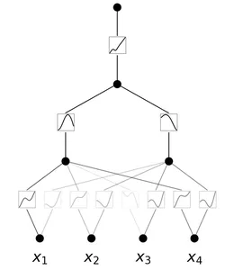
A Kolmogorov-Arnold Network is a neural network with learnable activation functions. At each node, the network learns the activation function. Unlike MLPs with fixed node activation functions, KANs have learnable activation functions on edges. They replace the linear weights with parametrized splines.
Advantages of KANs
Here are the advantages of KANs:
- Greater Flexibility: KANs are highly flexible due to their activation functions and model architecture, thus allowing better representation of complex data.
- Adaptable Activation Functions: Unlike in MLPs, the activation functions in KANs aren’t fixed. Since their activation functions are learnable on edges, they can adapt and adjust to different data patterns, thus effectively capturing diverse relationships.
- Better Complexity Handling: They replace the linear weights in MLPs by parametrized splines, thus they can handle complex, non-linear data.
- Superior Accuracy: KANs have demonstrated better accuracy in handling high-dimensional data
- Highly Interpretable: They reveal the structures and topological relationships between the data thus they can easily be interpreted.
- Diverse Applications: they can perform various tasks like regression, partial differential equations solving, and continual learning.
Also read: Multi-Layer Perceptrons: Notations and Trainable Parameters
Simple Implementation of KANs
Let’s implement KANs with the help of a simple example. We are going to create a custom dataset of the function: f(x, y) = exp(cos(pi*x) + y^2). This function takes two inputs, calculates the cosine of pi*x, adds the square of y to it, and then calculates the exponential of the result.
Requirements of Python library version:
- Python==3.9.7
- matplotlib==3.6.2
- numpy==1.24.4
- scikit_learn==1.1.3
- torch==2.2.2
!pip install git+https://github.com/KindXiaoming/pykan.git

import torch
import numpy as np

##create a dataset
def create_dataset(f, n_var=2, n_samples=1000, split_ratio=0.8):

    # Generate random input data
    X = torch.rand(n_samples, n_var)

    # Compute the target values
    y = f(X)

    # Split into training and test sets
    split_idx = int(n_samples * split_ratio)
    train_input, test_input = X[:split_idx], X[split_idx:]
    train_label, test_label = y[:split_idx], y[split_idx:]

    return {
        'train_input': train_input,
        'train_label': train_label,
        'test_input': test_input,
        'test_label': test_label
    }

# Define the new function f(x, y) = exp(cos(pi*x) + y^2)
f = lambda x: torch.exp(torch.cos(torch.pi*x[:, [0]]) + x[:, [1]]**2)

dataset = create_dataset(f, n_var=2)

print(dataset['train_input'].shape, dataset['train_label'].shape)
##output: torch.Size([800, 2]) torch.Size([800, 1])


from kan import *
# create a KAN: 2D inputs, 1D output, and 5 hidden neurons.
# cubic spline (k=3), 5 grid intervals (grid=5).
model = KAN(width=[2,5,1], grid=5, k=3, seed=0)

# plot KAN at initialization
model(dataset['train_input']);
model.plot(beta=100)
## train the model

model.train(dataset, opt="LBFGS", steps=20, lamb=0.01, lamb_entropy=10.)
## output: train loss: 7.23e-02 | test loss: 8.59e-02
## output: | reg: 3.16e+01 : 100%|██| 20/20 [00:11<00:00,  1.69it/s]

model.plot()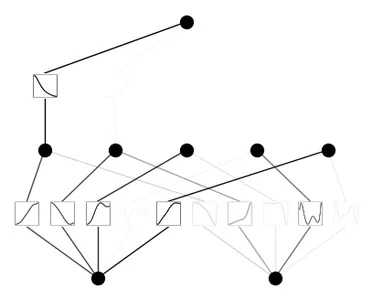
model.prune()
model.plot(mask=True)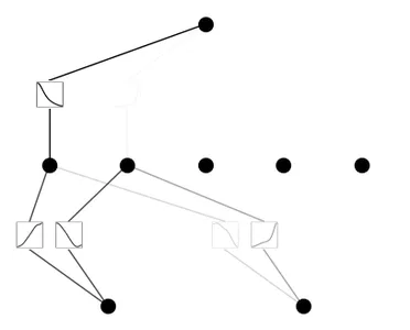
model = model.prune()
model(dataset['train_input'])
model.plot()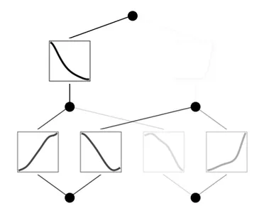
model.train(dataset, opt="LBFGS", steps=100)
model.plot()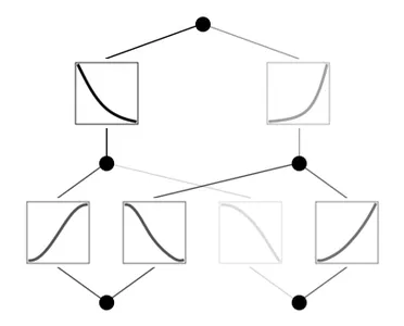
Code Explanation
- Install the Pykan library from Git Hub.
- Import libraries.
- The create_dataset function generates random input data (X) and computes the target values (y) using the function f. The dataset is then split into training and test sets based on the split ratio. The parameters of this function are:
- f: function to generate the target values.
- n_var: number of input variables.
- n_samples: total number of samples
- split_ratio: ratio to split the dataset into training and test sets, and it returns a dictionary containing training and test inputs and labels.
- Create a function of the form: f(x, y) = exp(cos(pi*x) + y^2)
- Call the function create_dataset to create a dataset using the previously defined function f with 2 input variables.
- Print the shape of training inputs and their labels.
- Initialize a KAN model with 2-dimensional inputs, 1-dimensional output, 5 hidden neurons, cubic spline (k=3), and 5 grid intervals (grid=5)
- Plot the KAN model at initialization.
- Train the KAN model using the provided dataset for 20 steps using the LBFGS optimizer.
- After training, plot the trained model.
- Prune the model and plot the pruned model with the masked neurons.
- Prune the model again, evaluate it on the training input, and plot the pruned model.
- Re-train the pruned model for an additional 100 steps.
MLP vs KAN
| MLP | KAN |
| Fixed node activation functions | Learnable activation functions |
| Linear weights | Parametrized splines |
| Less interpretable | More interpretable |
| Less flexible and adaptable as compared to KANs | Highly flexible and adaptable |
| Faster training time | Slower training time |
| Based on Universal Approximation Theorem | Based on Kolmogorov-Arnold Representation Theorem |
Conclusion
The invention of KANs indicates a step towards advancing deep learning techniques. By providing better interpretability and accuracy than MLPs, they can be a better choice when interpretability and accuracy of the results are the main objective. However, MLPs can be a more practical solution for tasks where speed is essential. Research is continuously happening to improve these networks, yet for now, KANs represent an exciting alternative to MLPs.
Key Takeaways
- KANs are a new type of neural network with learnable activation functions on edges based on the Kolmogorov-Arnold representation theorem.
- KANs provide greater flexibility and adaptability, better handling of complex data, superior accuracy, and higher interpretability than MLPs.
- The blog details how to implement KANs in Python, including dataset creation, model initialization, training, and visualization.
- KANs differ from MLPs by having learnable activation functions and parametrized splines, making them more interpretable but slower to train.
- KANs represent an advanced alternative to MLPs, particularly when accuracy and interpretability are prioritized over training speed.
The media shown in this article are not owned by Analytics Vidhya and is used at the Author’s discretion.
Frequently Asked Questions
Q1. Who invented KANs?
A. Ziming Liu, Yixuan Wang, Sachin Vaidya, Fabian Ruehle, James Halverson, Marin Soljaci, Thomas Y. Hou, Max Tegmark are the researchers involved in the dQevelopment of KANs.
Q2. What are fixed and learnable activation functions?
A. Fixed activation functions are mathematical functions applied to the outputs of neurons in neural networks. These functions remain constant throughout training and are not updated or adjusted based on the network’s learning. Ex: Sigmoid, tanh, ReLU.
Learnable activation functions are adaptive and modified during the training process. Instead of being predefined, they are updated through backpropagation, allowing the network to learn the most suitable activation functions.
Q3. What are some limitations of KANs as compared to MLPs?
A. One limitation of KANs is their slower training time due to their complex architecture. They require more computations during the training process since they replace the linear weights with spline-based functions that require additional computations to learn and optimize.
Q4. How do you choose between KANs or MLPs?
A. If your task requires more accuracy and interpretability and training time isn’t limited, you can proceed with KANs. If training time is critical, MLPs are a practical option.
Q5. What is an LBFGS optimizer?
A. The LBFGS optimizer stands for “Limited-memory Broyden–Fletcher–Goldfarb–Shanno” optimizer. It is a popular algorithm for parameter estimation in machine learning and numerical optimization.
Hello data enthusiasts! I am V Aditi, a rising and dedicated data science and artificial intelligence student embarking on a journey of exploration and learning in the world of data and machines. Join me as I navigate through the fascinating world of data science and artificial intelligence, unraveling mysteries and sharing insights along the way! 📊✨


