How to Compute and Store Vector Embeddings with LangChain?

Introduction

In our previous articles, we have discussed loading different types of data and different ways of splitting that data. The data is split to find the relevant content to the query from all the data. Now, we’re leaping into the future of data retrieval. This article will explore the cutting-edge technique of using vector embeddings with LangChain to find content that closely matches your query efficiently. Join us as we uncover how this powerful approach transforms data handling, making searches faster, more accurate, and intuitive.

Overview

• Learn the fundamentals of text embeddings, including representing words and sentences as numerical vectors to capture semantic meanings.
• Gain practical experience using LangChain’s and hugging face embedding models to compute and compare sentence embeddings.
• Explore how to efficiently store and retrieve relevant documents using vector databases using Approximate Nearest Neighbor algorithms.
• Understand LangChain’s indexing modes and learn to effectively manage document updates and deletions to maintain an optimal vector database.

Sentence Embeddings

Before using embedding models from LangChain, let’s briefly review what embeddings are in the context of text. 

To perform any computation with the text, we need to convert it into numerical form. Since all words are inherently related to each other, we can represent them as vectors of numbers that capture their semantic meanings. For example, the distance between the vectors representing two synonyms is smaller for synonyms and higher for antonyms. This is typically done using models like BERT.

Since the number of sentences is vastly higher than the number of words, we can’t calculate the embeddings for each sentence in the way we calculate the word embeddings. Sentence embeddings are calculated using SentenceBERT models, which use the Siamese network. For more details, read Sentence Embedding.

Let’s Create LangChain Documents

Requirements

Install langchain_openai, langchain-huggingface, and langchain-chroma packages using pip in addition to langchain and langchain_community libraries. Make sure to add the OpenAI API key to use OpenAI embedding models.

pip install langchain_openai langchain-huggingface langchain-chroma langchain langchain_community

Example: Creating LangChain Documents

I am using a few example sentences and a query sentence to explain the topics in this article. Later, let us also create LangChain documents using the sentences and categories.

from langchain_core.documents import Document
sentences = [
    "The Milky Way galaxy contains billions of stars, each potentially hosting its own planetary system.",
    "Photosynthesis is a process used by plants to convert light energy into chemical energy.",
    "The principles of supply and demand are fundamental to understanding market economies.",
    "In calculus, the derivative represents the rate of change of a function with respect to a variable.",
    "Quantum mechanics explores the behavior of particles at the smallest scales, where classical physics no longer applies.",
    "Enzymes are biological catalysts that speed up chemical reactions in living organisms.",
    "Game theory is a mathematical framework used for analyzing strategic interactions between rational decision-makers.",
    "The double helix structure of DNA was discovered by Watson and Crick in 1953, revolutionizing biology."
]
categories = ["Astronomy", "Biology", "Economics", "Mathematics", "Physics", "Biochemistry", "Mathematics", "Biology"]
query = 'Plants use sunlight to create energy through a process called photosynthesis.'
documents = []
for i, sentence in enumerate(sentences):
    documents.append(Document(page_content=sentence, metadata={'source': categories[i]}))
# creating Documents with metadata where 'source' is the category
# The documents will be as follows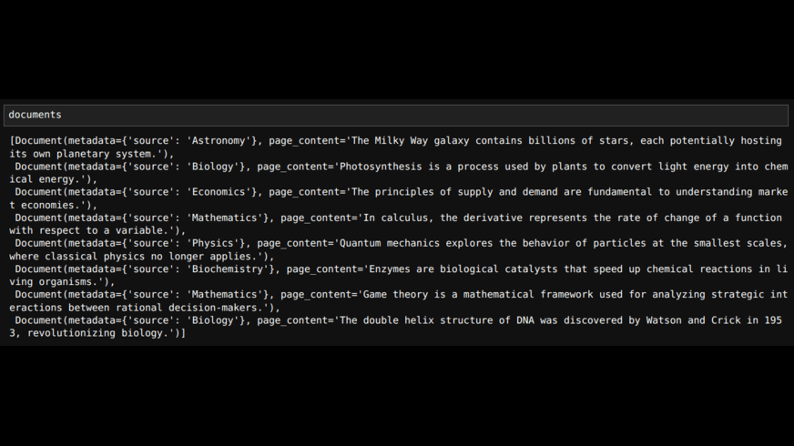

Embeddings with LangChain

Let us initialize the embedding model and embed the sentences.

import os
from dotenv import load_dotenv
load_dotenv(api_keys.env)

from langchain_openai import OpenAIEmbeddings
embedding_model = OpenAIEmbeddings(model='text-embedding-3-small', show_progress_bar=True)
embeddings = embedding_model.embed_documents(sentences)
# check the total number of embeddings and embedding dimension
len(embeddings)
>>> 8
len(embeddings[0])
>>> 1536

Now, let’s calculate the cosine similarity of sentences with each other and plot them as heat maps.

import numpy as np
import seaborn as sns
from sklearn.metrics.pairwise import cosine_similarity
similarities = cosine_similarity(embeddings)
sns.heatmap(similarities, cmap='magma', center=None, annot=True, fmt='.2f', yticklabels=sentences)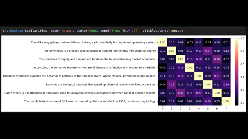

As we can see, sentences that belong to the same category and are similar to each other have a higher correlation to each other than with others.

Let’s compute the cosine similarities of these sentences w.r.t. the query sentence. We can find the most similar sentence to the query sentence.

query_embedding = embedding_model.embed_query(query)
query_similarities = cosine_similarity(X=[query_embedding], Y=embeddings)
#arrange the sentences in the descending order of their similarity with query sentence
for i in np.argsort(similarities[0])[::-1]:
    print(format(query_similarities[0][i], '.3f'), sentences[i])
"0.711 Photosynthesis is a process used by plants to convert light energy into chemical energy.
0.206 Enzymes are biological catalysts that speed up chemical reactions in living organisms.
0.172 The Milky Way galaxy contains billions of stars, each potentially hosting its own planetary system.
0.104 The double helix structure of DNA was discovered by Watson and Crick in 1953, revolutionizing biology.
0.100 Quantum mechanics explores the behavior of particles at the smallest scales, where classical physics no longer applies.
0.098 The principles of supply and demand are fundamental to understanding market economies.
0.067 Game theory is a mathematical framework used for analyzing strategic interactions between rational decision-makers.
0.053 In calculus, the derivative represents the rate of change of a function with respect to a variable.""

We can run them locally because embedding models require much less computing power than LLMs. Let’s run an open-source embedding model. We can compare and choose models from Huggingface.

from langchain_huggingface import HuggingFaceEmbeddings
hf_embedding_model = HuggingFaceEmbeddings(model_name='Snowflake/snowflake-arctic-embed-m')
embeddings = hf_embedding_model.embed_documents(sentences)
len(embeddings)
>>> 8
len(embeddings[0])
>>> 768

We can calculate the query embeddings and compute similarities with sentences as we have done above.

An important thing to note is each embedding model is likely trained on different data, so the vector embeddings of each model are likely in different vector spaces. So, if we embed the sentences and query with different embedding models, the results can be inaccurate even if the embedding dimensions are the same.

Using Vector Store

In the above example of finding similar sentences, we have compared the query embedding with each sentence embedding. However, if we have to find relevant documents from millions of documents, comparing query embedding with each will take a lot of time. We can use approximate nearest neighbors algorithms using a vector database to find the most efficient solution. To find out how those algorithms work, please refer to ANN Algorithms in Vector Databases.

Let us store the above example sentences in the vector store.

from langchain_chroma import Chroma
db = Chroma.from_texts(texts=sentences, embedding=embedding_model, persist_directory='./sentences_db',
                       collection_name='example', collection_metadata={"hnsw:space": "cosine"})        

Code explanation

1. Chroma.from_texts: This is to create a database using texts. Chroma.from_documents can be used to use LangChain documents.
2. embedding: This is an embedding model loaded through LangChain.
3. persist_directory: By adding a location, we can save the database to load it later and avoid computing embeddings again.
4. collection_name: Name for the collection of documents we are storing. Make sure the directory name and collection name are different.
5. collection_metadata: This specifies the distance metric used for comparing embeddings. Other options are ‘l2’ (l2 norm) and ‘ip’ (inner product)

Some of the methods we can use on the database are as follows

# this will get the ids of the documents
ids = db.get()['ids']
# can used to get other data about the documents
db.get(include=['embeddings', 'metadatas', 'documents'])
# this can be used to delete documents by id.
db._collection.delete(ids=ids)
# this is to delete the collection
db.delete_collection()

Now, we can search the database with the query and get the distance between the query embedding and sentences.

db.similarity_search_with_score(query=query, k=3)
# the above will get the documents with distance metric. 
# If we want similarity scores we can use
db.similarity_search_with_relevance_scores(query=query, k=3)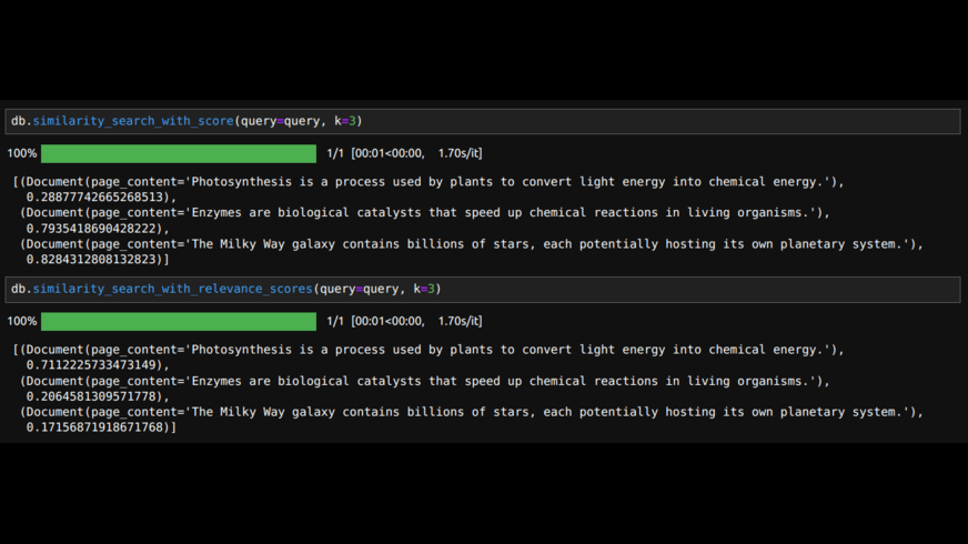

To get the relevance scores within 0 to 1 for the ‘l2’ distance metric, we need to pass the relevance_score_fn

db = Chroma.from_texts(texts=sentences, embedding=embedding_model, relevance_score_fn=lambda distance: 1.0 - distance / 2,
                       collection_name='sentences', collection_metadata={"hnsw:space": "l2"})

In the above code, we have only used the LangChain library. We can also directly use chromadb as follows:

import chromadb
from chromadb.utils.embedding_functions import OpenAIEmbeddingFunction

embedding_function = OpenAIEmbeddingFunction(api_key=os.environ.get('OPENAI_API_KEY'), model_name='text-embedding-3-small')
# initialize the client
client = chromadb.PersistentClient('./sentence_db')
# create a collection if it didn't exist otherwise load it
collection = client.get_or_create_collection('example', metadata={'hnsw:space': 'cosine'}, embedding_function=embedding_function)
# add sentences with any ids
collection.add(ids=ids, documents=sentences)

# now initialize the database collection to query
db = Chroma(client=client, collection_name='example', embedding_function=embedding_model)
# note that the embedding_function parameter here needs the embedding model loaded using langchain

Loading the vector database from a saved directory is as follows:

db2 = Chroma(persist_directory="./sentences_db/", collection_name='example', embedding_function=embedding_model)

# make sure you mention the collection name that you have used while creating the database.

# we can search this database as we have previously.

Sometimes, we may accidentally run the add documents code again, which will add the same documents to the database, creating unnecessary duplicates. We may also need to update some documents and delete all but a few.

For all of that, we can use Indexing API from LangChain

Indexing

LangChain indexing uses a Record Manager to track document entries in the vector store. Therefore, we can’t use Indexing for an existing database, as the record manager doesn’t track the database’s existing content.

When content is indexed, hashes are computed for each document, and the following information is stored in the Record Manager.

• Document Hash: A hash of both the page content and its metadata.
• Write Time: The timestamp when the document was written.
• Source ID: Metadata that includes information to identify the ultimate source of the document.

Using those, we can avoid re-writing and re-computing embeddings over unchanged content. There are three modes of Indexing. None, Incremental, Full:

1. None mode avoids writing duplicate content to the vector store and doesn’t update or delete anything.
2. Incremental mode updates the database with new content and deletes old content for a given source.
3. Full mode deletes any content not found in the currently indexed content.

The categories we added as sources in the metadata when creating documents will be useful here.

from langchain.indexes import SQLRecordManager, index

# initialize the database
db = Chroma(persist_directory='./sentence_db', collection_name='example', 
            embedding_function=embedding_model, collection_metadata={"hnsw:space": "cosine"})
# name a namespace that indicates database and collection
namespace = f"db/example"

record_manager = SQLRecordManager(namespace, db_url="sqlite:///record_manager.sql")
record_manager.create_schema()

# load and index the documents 
index(docs_source=documents, record_manager=record_manager, vector_store=db, cleanup=None)
>>> {'num_added': 8, 'num_updated': 0, 'num_skipped': 0, 'num_deleted': 0}

If we run the last line of code again, we will see num_skipped as 8 and all others as 0.

doc1 = Document(page_content="The human immune system protects the body from infections by identifying and destroying pathogens", 
                metadata={"source": "Biology"})
doc2 = Document(page_content="Genetic mutations can lead to variations in traits, which may be beneficial, neutral, or harmful", 
                metadata={"source": "Biology"})
# add these docs to the database in incremental mode
index(docs_source=[doc1, doc2], record_manager=record_manager, vector_store=db, cleanup='incremental', source_id_key='source')
>>> {'num_added': 2, 'num_updated': 0, 'num_skipped': 0, 'num_deleted': 0}

With the above code, both are added, and none are deleted, as the previous 8 documents are not added in incremental mode. If the previous 8 were added in incremental mode, then 2 documents would be deleted, and 2 would be added.

If we slightly change doc2 and rerun the indexing code, doc1 will be skipped as it is not changed, the existing doc2 will be deleted from the database, and the changed doc2 will be added. This is denoted as {‘num_added’: 1, ‘num_updated’: 0, ‘num_skipped’: 1, ‘num_deleted’: 1}

In the full mode, if we don’t mention any docs while indexing, all the existing docs will be deleted.

index([], record_manager=record_manager, vector_store=db, cleanup="full", source_id_key="source")
>>> {'num_added': 0, 'num_updated': 0, 'num_skipped': 0, 'num_deleted': 10}
# this will delete all the documents in database

So, by using different modes, we can efficiently manage what data to keep and what to update and delete. Practice this indexing with different combinations of modes to understand it better.

Conclusion

Here, we have demonstrated how to efficiently find content similar to a query using vector embeddings with LangChain. We can achieve accurate and scalable content retrieval by leveraging embedding models and vector databases. Additionally, LangChain’s indexing capabilities allow for effective management of document updates and deletions, ensuring optimal database performance and relevance.

In the next article, we will discuss different ways of retrieving the content to send to the LLM.

Frequently Asked Questions

Santosh 05 Aug, 2024

I am working as an Associate Data Scientist at Analytics Vidhya, a platform dedicated to building the Data Science ecosystem. My interests lie in the fields of Deep Learning and Natural Language Processing (NLP).