Introduction
Conditional Formatting in Excel is more than just a feature—it’s a powerful tool transforming how you interact with data. Whether you’re managing a simple budget or analyzing complex datasets, Conditional Formatting helps you highlight important trends, patterns, and outliers with just a few clicks. In this article, we’ll explore how you can utilize this feature to make your data more visually appealing and informative.

Overview
- Learn how Conditional Formatting in Excel turns raw data into visual insights, making trends and outliers stand out.
- Discover how to use Excel’s Conditional Formatting rules to automatically highlight critical data points with colors, icons, and data bars.
- Explore applying customized Conditional Formatting using Excel formulas for more nuanced data analysis.
- Use Conditional Formatting to spot top/bottom performers quickly and duplicate entries in large datasets.
- Gain practical tips to maximize the impact of Conditional Formatting without overwhelming your spreadsheets.
- Master Conditional Formatting to create visually appealing and informative spreadsheets that communicate data stories effectively.
Table of contents
Conditional Formatting: An Overview
At its core, Conditional Formatting allows you to apply specific formatting—such as colors, icons, or data bars—to cells based on the values they contain. This automatic formatting is triggered by rules you define, making it easy to spot critical data points or trends without manually sifting through numbers.
Also read: Microsoft Excel for Data Analysis
Highlighting Cells Based on Value
One of the simplest yet most effective uses of Conditional Formatting is highlighting cells based on their value. For instance, if you want to quickly identify which sales figures exceed a certain threshold, conditional formatting can help you. Here’s how:
Here’s how you can highlight cells based on values:
- Select the Range
Choose the cells you want to format.

- Navigate to Conditional Formatting
Find the Conditional Formatting option on the Home tab under the Styles group.

- Choose Your Rule
Select “Highlight Cells Rules” and then “Greater Than.” Then, Enter the threshold value and choose your desired formatting style.

- Apply the Formatting
Click OK, and Excel will highlight the cells that meet your criteria.

Using Formulas for Custom Formatting
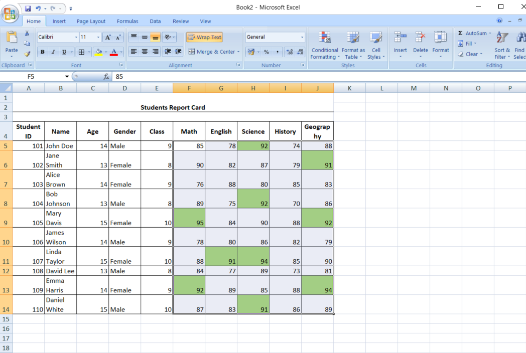
Excel’s flexibility shines when you use formulas to apply Conditional Formatting. This allows for more nuanced and customized rules. For example, you might want to highlight cells based on a condition that isn’t simply a comparison to a static value, like flagging sales higher than the previous month’s average.
- Select Your Range: Highlight the cells you want to format.
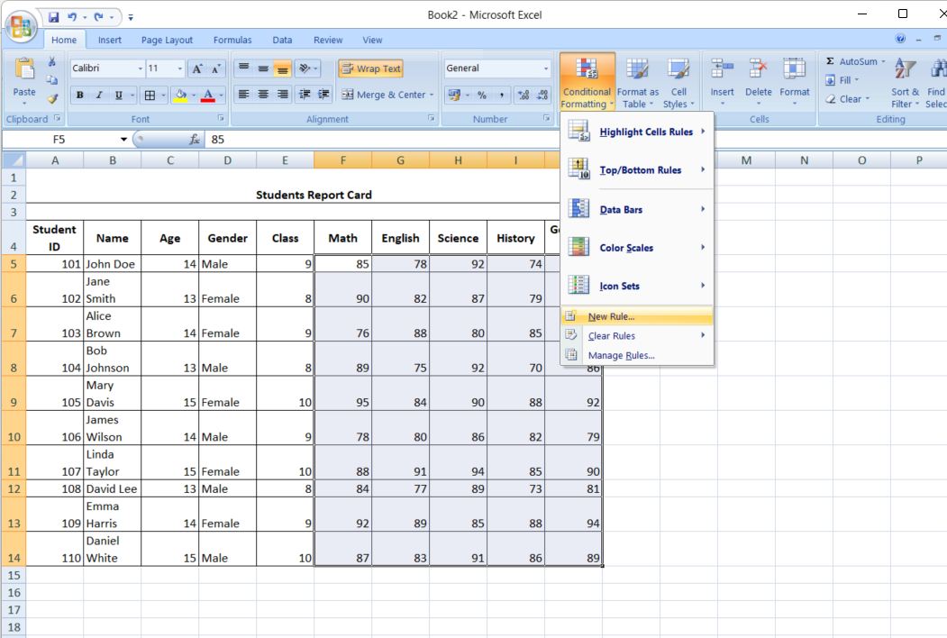
- Create a New Rule: Under the Conditional Formatting menu, select “New Rule” and choose “Use a formula to determine which cells to format.”
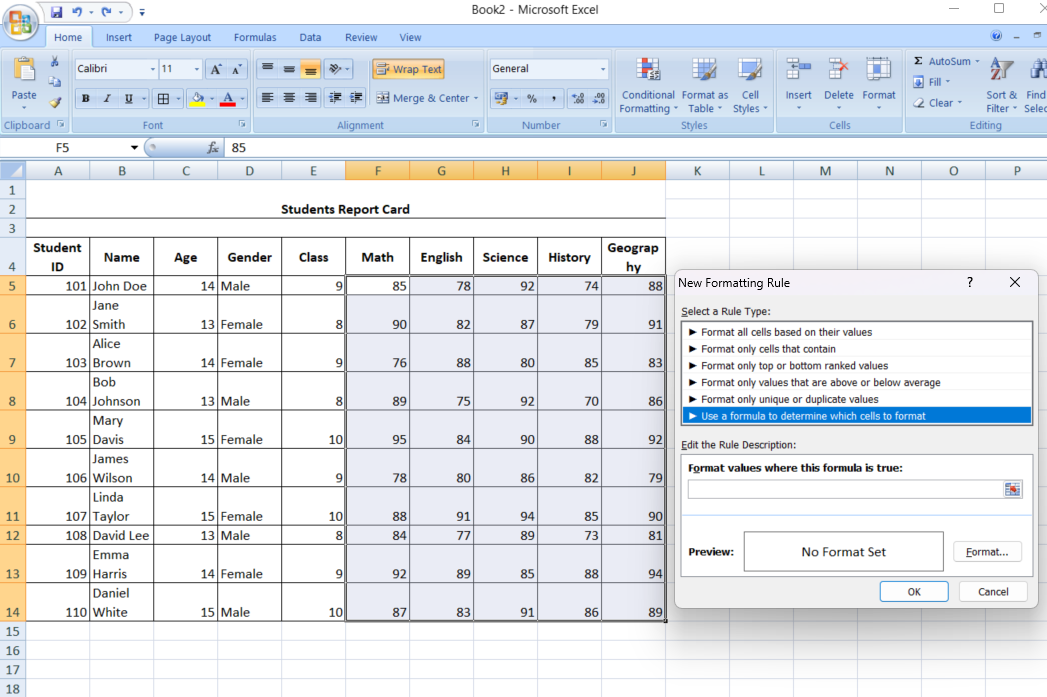
- Input the Formula: Enter your formula, which should return a TRUE or FALSE outcome.
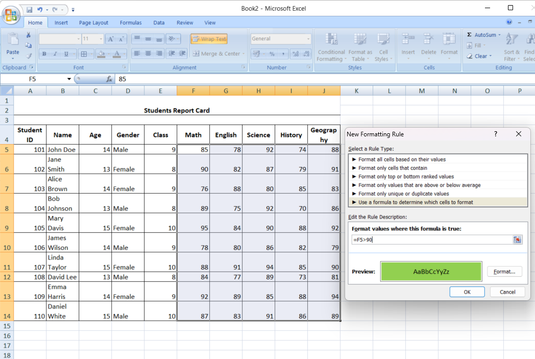
- Select a Format: Choose how you want the cells to appear if the condition is met.
- Apply: Hit OK to see the changes in your spreadsheet.
Also read: A Comprehensive Guide on Advanced Microsoft Excel for Data Analysis.
Highlighting Extremes: Top/Bottom Rules
Conditional Formatting can also help you focus on the highest and lowest values in a dataset, such as identifying the top 10 performers or the bottom 5 sales figures.
- Select Your Data Range: Highlight the relevant cells.
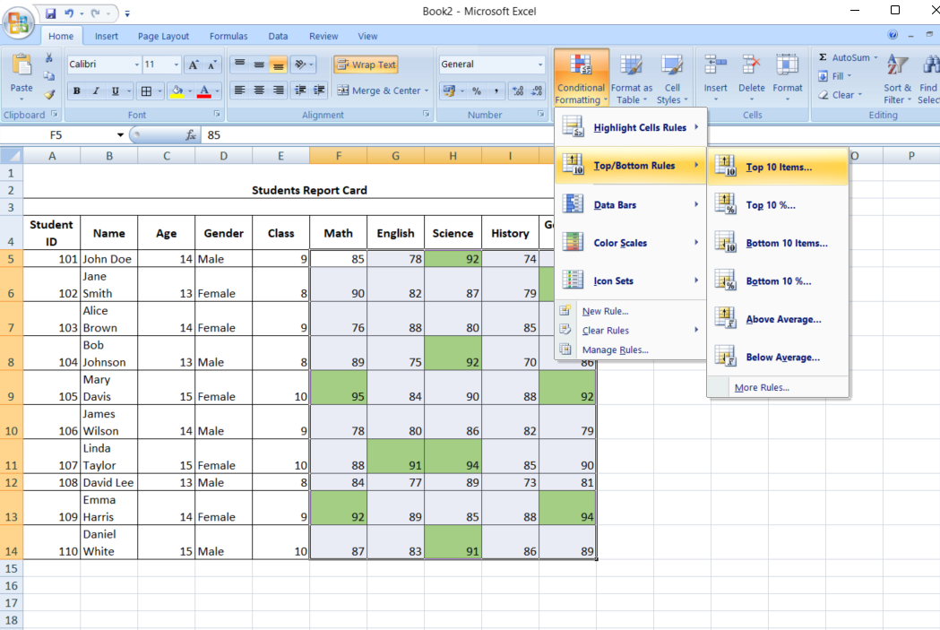
- Access Conditional Formatting: Navigate to Conditional Formatting > Top/Bottom Rules.
- Set the Parameters: Select whether to highlight the top or bottom values and specify the number of items.
- Finalize the Formatting: Select the desired formatting style and apply the rule.
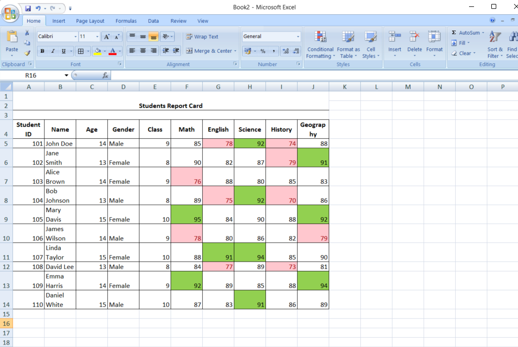
Similarly, identifying duplicate entries is crucial in large datasets. Conditional Formatting can quickly highlight duplicates, helping you maintain data accuracy.
- Select the Range: Choose the cells you want to check for duplicates.
- Choose Duplicate Values Rule: Under the Conditional Formatting menu, select “Highlight Cells Rules” and “Duplicate Values.”
- Apply Formatting: Pick the formatting style and click OK.
Tips for Effective Use of Conditional Formatting in Excel
Here are the tips:
- Start Simple: Begin with basic rules like highlighting values greater than or less than a specific number. This will help you get comfortable with how Conditional Formatting works.
- Use Cell References for Flexibility: Instead of using static values in your Conditional Formatting rules, refer to another cell. This allows you to change the criteria by simply updating the reference cell.
- Leverage Formulas for Custom Rules: Excel’s formula-based Conditional Formatting lets you create highly customized rules. Ensure that your formula returns a TRUE or FALSE value to apply the formatting correctly.
- Combine Multiple Rules: Don’t hesitate to apply multiple Conditional Formatting rules to the same range of cells. For example, you can use both Color Scales and Icon Sets to provide different layers of data insight.
- Review and Manage Rules Regularly: As you add more Conditional Formatting, check and manage your rules to avoid conflicts or overly complex setups. Use the “Manage Rules” option to edit or delete rules as needed.
- Prioritize Rules: When applying multiple rules, remember that Excel prioritizes them in the order they are listed. You can change the priority by moving rules up or down in the “Manage Rules” dialogue.
- Use Preview to Your Advantage: Before applying conditional formatting, use the preview function to see how your data will look. This helps you tweak the settings for the best visual result.
- Avoid Overloading with Formatting: While Conditional Formatting is powerful, too much can overwhelm your spreadsheet and make it difficult to read. Use formatting sparingly to ensure clarity.
- Experiment with Custom Formats: Excel allows you to create custom formatting styles (e.g., specific colors or font styles) in Conditional Formatting. This is particularly useful for maintaining a consistent look across your spreadsheets.
- Clear Formatting When Needed: If your data changes significantly, clear the old formatting rules to start fresh. This prevents outdated rules from applying incorrectly to new data.
Conclusion
Conditional Formatting in Excel is not just a handy feature—it’s a game-changer for anyone who works with data. By leveraging this tool, you can turn a simple spreadsheet into a dynamic, visually appealing report highlighting key insights and trends at a glance. Whether you’re a data novice or an experienced analyst, mastering Conditional Formatting will enhance your ability to communicate data-driven stories effectively. So, the next time you’re in Excel, don’t just look at the numbers—let Conditional Formatting help you see the bigger picture.
Frequently Asked Questions
Q1. What is Conditional Formatting?
Ans. Conditional Formatting in Excel lets you apply specific formatting to cells based on their values, such as highlighting, color scales, or icon sets.
Q2. How do I apply Conditional Formatting?
Ans. Select the cells, go to the “Home” tab, click “Conditional Formatting,” choose a rule, and configure it as needed.
Q3. Can I use formulas with Conditional Formatting?
Ans. Yes, you can use formulas to create custom Conditional Formatting rules by selecting “Use a formula to determine which cells to format.”
Q4. How do I remove Conditional Formatting?
Ans. Select the cells, go to “Conditional Formatting” in the “Home” tab, and choose “Clear Rules” to remove the formatting.
Hi, I am Pankaj Singh Negi - Senior Content Editor | Passionate about storytelling and crafting compelling narratives that transform ideas into impactful content. I love reading about technology revolutionizing our lifestyle.


