Introduction
Artificial intelligence has revolutionized because of Stable Diffusion, which makes producing high-quality images from noise or text descriptions possible. Several essential elements come together in this potent generative model to create amazing visual effects. The five main components of Diffusion Models—the forward and reverse processes, the noise schedule, positional encoding, and neural network architecture—will all be covered in this article.
We will implement components of diffusion models as we go through the article. We will be using the Fashion MNIST Dataset for this.

Overview
- Discover how Stable Diffusion transforms AI image generation, bringing high-quality visuals from mere noise or text descriptions.
- Learn how images degrade to noise, training AI models to master the art of visual reconstruction.
- Explore how AI reconstructs high-quality images from noise, reversing the degradation process step by step.
- Understand the role of unique vector representations in guiding AI through varying noise levels during image generation.
- Delve into the symmetrical encoder-decoder structure of UNet, which excels at producing fine details and global structures.
- Examine the critical noise schedule in diffusion models, balancing generation quality and computational efficiency for high-fidelity AI outputs.
Table of contents
Forward Diffusion Process
The forward process is the initial stage of Stable Diffusion, where an image is gradually transformed into noise. This process is crucial for training the model to understand how images degrade over time.
Important aspects of the forward process consist of:
- Gaussian noise is gradually added to the image by the model over several timesteps in tiny increments.
- The Markov property states that every step in a forward process only depends on the step before it, creating a Markov chain.
- Gaussian convergence: The data distribution converges to a Gaussian distribution after a sufficient number of steps.
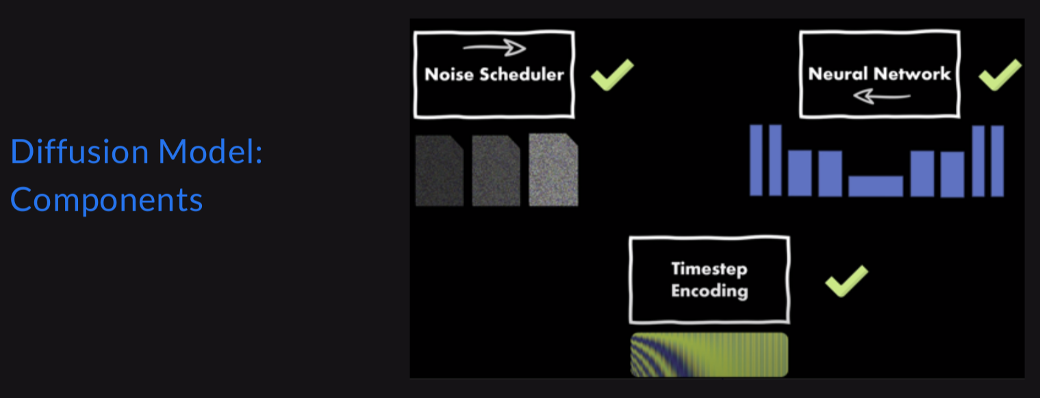
Here are the components of the diffusion model:
Implementation of the Forward Diffusion Process
The code in this notebook is adapted from Brian Pulfer’s DDPM implementation in his GitHub repo.
Importing necessary libraries
# Import of libraries

import random

import imageio

import numpy as np

from argparse import ArgumentParser

from tqdm.auto import tqdm

import matplotlib.pyplot as plt

import einops

import torch

import torch.nn as nn

from torch.optim import Adam

from torch.utils.data import DataLoader

from torchvision.transforms import Compose, ToTensor, Lambda

from torchvision.datasets.mnist import MNIST, FashionMNIST

# Setting reproducibility

SEED = 0

random.seed(SEED)

np.random.seed(SEED)

torch.manual_seed(SEED)

# Definitions

STORE_PATH_MNIST = f"ddpm_model_mnist.pt"

STORE_PATH_FASHION = f"ddpm_model_fashion.pt"
Setting SEED for reproducibility
no_train = False

fashion = True

batch_size = 128

n_epochs = 20

lr = 0.001

store_path = "ddpm_fashion.pt" if fashion else "ddpm_mnist.pt"
Setting some parameters, no_train is set to False. This implies that we will train the model, and not use any pretrained model. Batch_size, n_epochs, and lr are general deep-learning parameters. We will be using the Fashion MNIST dataset here.
Loading Data
# Loading the data (converting each image into a tensor and normalizing between [-1, 1])

transform = Compose([

   ToTensor(),

   Lambda(lambda x: (x - 0.5) * 2)]

)

ds_fn = FashionMNIST if fashion else MNIST

dataset = ds_fn("./datasets", download=True, train=True, transform=transform)

loader = DataLoader(dataset, batch_size, shuffle=True)
We will use the pytorch data loader to load our Fashion MNIST Dataset.
Forward Diffusion Process function
def forward(self, x0, t, eta=None):

       n, c, h, w = x0.shape

       a_bar = self.alpha_bars[t]

       if eta is None:

           eta = torch.randn(n, c, h, w).to(self.device)

       noisy = a_bar.sqrt().reshape(n, 1, 1, 1) * x0 + (1 - a_bar).sqrt().reshape(n, 1, 1, 1) * eta

       return noisy
The above function implements the forward diffusion equation directly to the desired step. Note: Here, we do not induce noise at each timestep; instead, we read the image at the timestep directly.
def show_forward(ddpm, loader, device):

   # Showing the forward process

   for batch in loader:

       imgs = batch[0]

       show_images(imgs, "Original images")

       for percent in [0.25, 0.5, 0.75, 1]:

           show_images(

               ddpm(imgs.to(device),

                    [int(percent * ddpm.n_steps) - 1 for _ in range(len(imgs))]),

               f"DDPM Noisy images {int(percent * 100)}%"

           )

       break
The above code will help us visualize the image noise at different levels: 25%, 50%, 75%, and 100%.
Reverse Diffusion Process
The core of stable diffusion is the reverse process, which teaches the model to piece together noisy images into high-quality ones. This process, employed for training and image generation, is the opposite of the forward process.
Important aspects of the opposite procedure:
- Iterative denoising: The original image is progressively revealed as the model gradually removes the noise.
- Noise prediction: The model makes predictions about the noise in the current image at each step.
- Controlled generation: More control over the creation of images is possible thanks to the reverse process, which permits interventions at particular timesteps.
Also Read: Unraveling the Power of Diffusion Models in Modern AI
Implementation of Reverse Diffusion Process
def backward(self, x, t):

       # Run each image through the network for each timestep t in the vector t.

       # The network returns its estimation of the noise that was added.

       return self.network(x, t)
Well you may say that the reverse diffusion process function is very simple, it is because in reverse diffusion the network (we will look into the network part soon) predicts the amount of noise, calculates the loss with the original noise to learn. Hence, the code is very simple. Below is the code for the entire DDPM – Denoise Diffusion Probabilistic Model.
The below code creates a Denoising Diffusion Probabilistic Model (DDPM) and defines the MyDDPM PyTorch module. The forward diffusion process is implemented by the forward technique, which adds noise to an input image based on a predetermined timestep. The backward approach, essential for the reverse diffusion process, estimates the noise in a given noisy image at a particular timestep using a neural network. The class also initializes diffusion process parameters such as alpha and beta schedules.
# DDPM class

class MyDDPM(nn.Module):

   def __init__(self, network, n_steps=200, min_beta=10 ** -4, max_beta=0.02, device=None, image_chw=(1, 28, 28)):

       super(MyDDPM, self).__init__()

       self.n_steps = n_steps

       self.device = device

       self.image_chw = image_chw

       self.network = network.to(device)

       self.betas = torch.linspace(min_beta, max_beta, n_steps).to(

           device)  # Number of steps is typically in the order of thousands

       self.alphas = 1 - self.betas

       self.alpha_bars = torch.tensor([torch.prod(self.alphas[:i + 1]) for i in range(len(self.alphas))]).to(device)

   def forward(self, x0, t, eta=None):

       # Make input image more noisy (we can directly skip to the desired step)

       n, c, h, w = x0.shape

       a_bar = self.alpha_bars[t]

       if eta is None:

           eta = torch.randn(n, c, h, w).to(self.device)

       noisy = a_bar.sqrt().reshape(n, 1, 1, 1) * x0 + (1 - a_bar).sqrt().reshape(n, 1, 1, 1) * eta

       return noisy

   def backward(self, x, t):

       # Run each image through the network for each timestep t in the vector t.

       # The network returns its estimation of the noise that was added.

       return self.network(x, t)
The parameters are n_steps, which tells us the number of timesteps in the training process. min_beta and max_beta indicate the noise schedule, which we will discuss soon.
def generate_new_images(ddpm, n_samples=16, device=None, frames_per_gif=100, gif_name="sampling.gif", c=1, h=28, w=28):

   """Given a DDPM model, a number of samples to be generated and a device, returns some newly generated samples"""

   frame_idxs = np.linspace(0, ddpm.n_steps, frames_per_gif).astype(np.uint)

   frames = []

   with torch.no_grad():

       if device is None:

           device = ddpm.device

       # Starting from random noise

       x = torch.randn(n_samples, c, h, w).to(device)

       for idx, t in enumerate(list(range(ddpm.n_steps))[::-1]):

           # Estimating noise to be removed

           time_tensor = (torch.ones(n_samples, 1) * t).to(device).long()

           eta_theta = ddpm.backward(x, time_tensor)

           alpha_t = ddpm.alphas[t]

           alpha_t_bar = ddpm.alpha_bars[t]

           # Partially denoising the image

           x = (1 / alpha_t.sqrt()) * (x - (1 - alpha_t) / (1 - alpha_t_bar).sqrt() * eta_theta)

           if t > 0:

               z = torch.randn(n_samples, c, h, w).to(device)

               # Option 1: sigma_t squared = beta_t

               beta_t = ddpm.betas[t]

               sigma_t = beta_t.sqrt()

               # Option 2: sigma_t squared = beta_tilda_t

               # prev_alpha_t_bar = ddpm.alpha_bars[t-1] if t > 0 else ddpm.alphas[0]

               # beta_tilda_t = ((1 - prev_alpha_t_bar)/(1 - alpha_t_bar)) * beta_t

               # sigma_t = beta_tilda_t.sqrt()

               # Adding some more noise like in Langevin Dynamics fashion

               x = x + sigma_t * z

           # Adding frames to the GIF

           if idx in frame_idxs or t == 0:

               # Putting digits in range [0, 255]

               normalized = x.clone()

               for i in range(len(normalized)):

                   normalized[i] -= torch.min(normalized[i])

                   normalized[i] *= 255 / torch.max(normalized[i])

               # Reshaping batch (n, c, h, w) to be a (as much as it gets) square frame

               frame = einops.rearrange(normalized, "(b1 b2) c h w -> (b1 h) (b2 w) c", b1=int(n_samples ** 0.5))

               frame = frame.cpu().numpy().astype(np.uint8)

               # Rendering frame

               frames.append(frame)

   # Storing the gif

   with imageio.get_writer(gif_name, mode="I") as writer:

       for idx, frame in enumerate(frames):

           # Convert grayscale frame to RGB

           rgb_frame = np.repeat(frame, 3, axis=-1)

           writer.append_data(rgb_frame)

           if idx == len(frames) - 1:

               for _ in range(frames_per_gif // 3):

                   writer.append_data(rgb_frame)

   return x
The above code is our function for generating new images. It creates 16 new images. The reverse process of those 16 new images is captured at each timestep, but only 100 are taken from 200 timesteps. Then, those 100 frames are turned into GIFs to show the visualization of our model-generating images.
The above code will be generated once the network is set. Now, let’s look into the neural network.
Also read: Implementing Diffusion Models for Creative AI Art Generation
Neural Network Architecture
Before we look into the architecture of our neural network, which we will use to generate images. We should know that the diffusion model’s parameters are shared across different timesteps. It must remove noise from images with widely different levels of noise. Hence, we have positional encoding, which encodes the timestep using a sinusoidal function to address this.
Implementation of Positional Encoding
Key aspects of positional encoding:
- Distinct representation: Each timestep is given a unique vector representation.
- Noise level awareness: Helps the model understand the current noise level, allowing for appropriate denoising decisions.
- Process guidance: Guides the model through different stages of the diffusion process.
def sinusoidal_embedding(n, d):

   # Returns the standard positional embedding

   embedding = torch.zeros(n, d)

   wk = torch.tensor([1 / 10_000 ** (2 * j / d) for j in range(d)])

   wk = wk.reshape((1, d))

   t = torch.arange(n).reshape((n, 1))

   embedding[:,::2] = torch.sin(t * wk[:,::2])

   embedding[:,1::2] = torch.cos(t * wk[:,::2])

   return embedding
Now that we have seen positional encoding to distinguish between timesteps, we will look into our Neural Network Architecture. UNet is the most common architecture used in the diffusion model because it works at the image’s pixel level. It features a symmetric encoder-decoder structure with skip connections between corresponding layers. In Stable Diffusion, U-Net predicts the noise at each denoising step. Its ability to capture and combine features at different scales makes it particularly effective for image generation tasks, allowing the model to maintain fine details and global structure in the generated images.
Let’s declare UNet for our stable diffusion process.
class MyUNet(nn.Module):

   '''

   Vanilla UNet Implementation with Timesteps Positional Ecndoing being used in every block in addition to Usual input from previous block

   '''

   def __init__(self, n_steps=1000, time_emb_dim=100):

       super(MyUNet, self).__init__()

       # Sinusoidal embedding

       self.time_embed = nn.Embedding(n_steps, time_emb_dim)

       self.time_embed.weight.data = sinusoidal_embedding(n_steps, time_emb_dim)

       self.time_embed.requires_grad_(False)

       # First half

       self.te1 = self._make_te(time_emb_dim, 1)

       self.b1 = nn.Sequential(

           MyBlock((1, 28, 28), 1, 10),

           MyBlock((10, 28, 28), 10, 10),

           MyBlock((10, 28, 28), 10, 10)

       )

       self.down1 = nn.Conv2d(10, 10, 4, 2, 1)

       self.te2 = self._make_te(time_emb_dim, 10)

       self.b2 = nn.Sequential(

           MyBlock((10, 14, 14), 10, 20),

           MyBlock((20, 14, 14), 20, 20),

           MyBlock((20, 14, 14), 20, 20)

       )

       self.down2 = nn.Conv2d(20, 20, 4, 2, 1)

       self.te3 = self._make_te(time_emb_dim, 20)

       self.b3 = nn.Sequential(

           MyBlock((20, 7, 7), 20, 40),

           MyBlock((40, 7, 7), 40, 40),

           MyBlock((40, 7, 7), 40, 40)

       )

       self.down3 = nn.Sequential(

           nn.Conv2d(40, 40, 2, 1),

           nn.SiLU(),

           nn.Conv2d(40, 40, 4, 2, 1)

       )

       # Bottleneck

       self.te_mid = self._make_te(time_emb_dim, 40)

       self.b_mid = nn.Sequential(

           MyBlock((40, 3, 3), 40, 20),

           MyBlock((20, 3, 3), 20, 20),

           MyBlock((20, 3, 3), 20, 40)

       )

       # Second half

       self.up1 = nn.Sequential(

           nn.ConvTranspose2d(40, 40, 4, 2, 1),

           nn.SiLU(),

           nn.ConvTranspose2d(40, 40, 2, 1)

       )

       self.te4 = self._make_te(time_emb_dim, 80)

       self.b4 = nn.Sequential(

           MyBlock((80, 7, 7), 80, 40),

           MyBlock((40, 7, 7), 40, 20),

           MyBlock((20, 7, 7), 20, 20)

       )

       self.up2 = nn.ConvTranspose2d(20, 20, 4, 2, 1)

       self.te5 = self._make_te(time_emb_dim, 40)

       self.b5 = nn.Sequential(

           MyBlock((40, 14, 14), 40, 20),

           MyBlock((20, 14, 14), 20, 10),

           MyBlock((10, 14, 14), 10, 10)

       )

       self.up3 = nn.ConvTranspose2d(10, 10, 4, 2, 1)

       self.te_out = self._make_te(time_emb_dim, 20)

       self.b_out = nn.Sequential(

           MyBlock((20, 28, 28), 20, 10),

           MyBlock((10, 28, 28), 10, 10),

           MyBlock((10, 28, 28), 10, 10, normalize=False)

       )

       self.conv_out = nn.Conv2d(10, 1, 3, 1, 1)

   def forward(self, x, t):

       # x is (N, 2, 28, 28) (image with positional embedding stacked on channel dimension)

       t = self.time_embed(t)

       n = len(x)

       out1 = self.b1(x + self.te1(t).reshape(n, -1, 1, 1))  # (N, 10, 28, 28)

       out2 = self.b2(self.down1(out1) + self.te2(t).reshape(n, -1, 1, 1))  # (N, 20, 14, 14)

       out3 = self.b3(self.down2(out2) + self.te3(t).reshape(n, -1, 1, 1))  # (N, 40, 7, 7)

       out_mid = self.b_mid(self.down3(out3) + self.te_mid(t).reshape(n, -1, 1, 1))  # (N, 40, 3, 3)

       out4 = torch.cat((out3, self.up1(out_mid)), dim=1)  # (N, 80, 7, 7)

       out4 = self.b4(out4 + self.te4(t).reshape(n, -1, 1, 1))  # (N, 20, 7, 7)

       out5 = torch.cat((out2, self.up2(out4)), dim=1)  # (N, 40, 14, 14)

       out5 = self.b5(out5 + self.te5(t).reshape(n, -1, 1, 1))  # (N, 10, 14, 14)

       out = torch.cat((out1, self.up3(out5)), dim=1)  # (N, 20, 28, 28)

       out = self.b_out(out + self.te_out(t).reshape(n, -1, 1, 1))  # (N, 1, 28, 28)

       out = self.conv_out(out)

       return out

   def _make_te(self, dim_in, dim_out):

       return nn.Sequential(

           nn.Linear(dim_in, dim_out),

           nn.SiLU(),

           nn.Linear(dim_out, dim_out)

       )
Instantiating the model
# Defining model

n_steps, min_beta, max_beta = 1000, 10 ** -4, 0.02  # Originally used by the authors

ddpm = MyDDPM(MyUNet(n_steps), n_steps=n_steps, min_beta=min_beta, max_beta=max_beta, device=device)

#Number of parameters in the model to be learned.

sum([p.numel() for p in ddpm.parameters()])
Visualization of Forward diffusion
show_forward(ddpm, loader, device)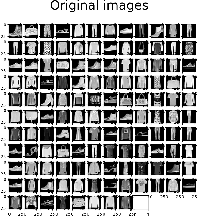
The above-mentioned images are original Fashion MNIST images without any noise. Here, we will take these images and slowly inducing noise into them.
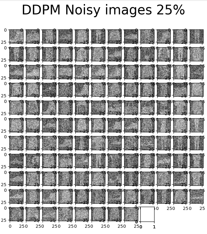
We can observe from the above-mentioned images that there is noise in the images, but it is not difficult to recognize them. We add noise as per our noise schedule. The above images contain 25% of the noise as per the linear noise schedule.
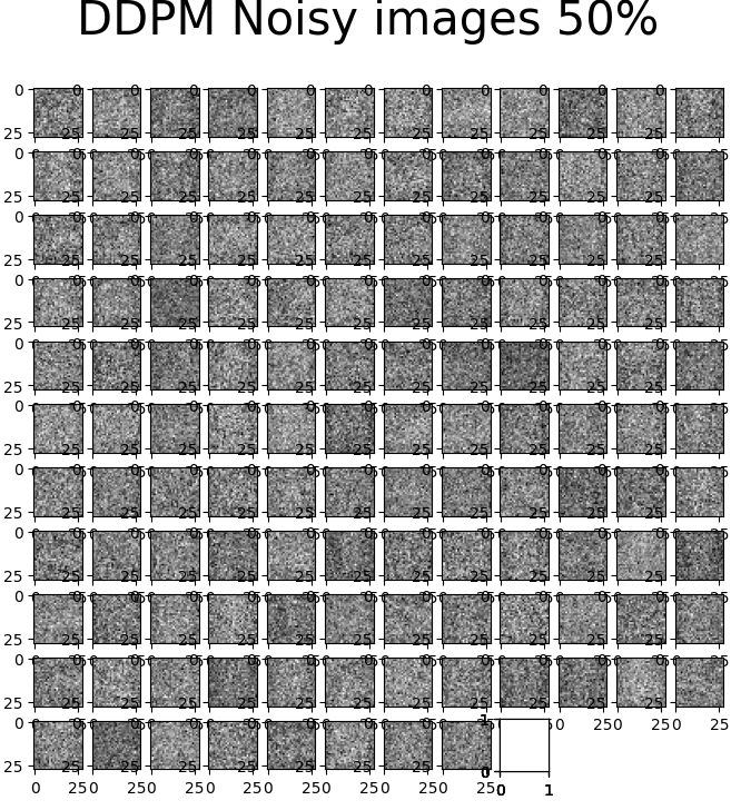
We can see that the noise is being gradually added until 100% of the image is noise. The above image shows 50% of the noise added as per noise schedule and at 50% we are unable to recognise images, this is considered a drawback of linear noise schedule and recent diffusion models use more advanced techniques to induce noise.
Generating Images Before Training
generated = generate_new_images(ddpm, gif_name="before_training.gif")
show_images(generated, "Images generated before training")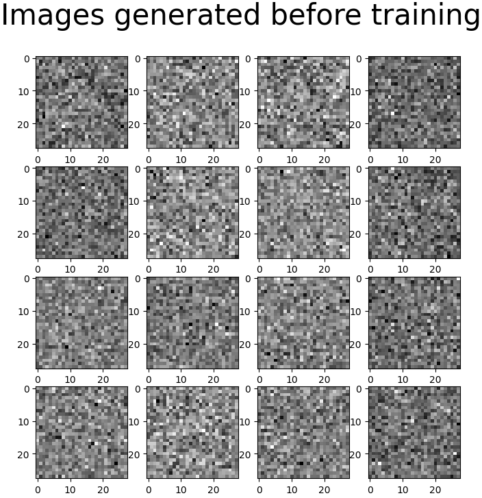
We can see that the model knows nothing about the dataset and can generate only noise. Before we start training our model, we will discuss the noise schedule.
Noise Schedule
The noise schedule is a critical component in diffusion models. It determines how noise is added during the forward process and removed during the reverse process. It also defines the rate at which information is destroyed and reconstructed, significantly impacting the model’s performance and the quality of generated samples.
A well-designed noise schedule balances the trade-off between generation quality and computational efficiency. Too rapid noise addition can lead to information loss and poor reconstruction, while too slow a schedule can result in unnecessarily long computation times. Advanced techniques like cosine schedules can optimize this process, allowing for faster sampling without sacrificing output quality. The noise schedule also influences the model’s ability to capture different levels of detail, from coarse structures to fine textures, making it a key factor in achieving high-fidelity generations.
In our DDPM model, we will use a Linear Schedule where noise is added linearly, but there are other recent advancements in Stable diffusion. Now that we understand the Noise schedule let’s train our model.
Model Training
In model training, we take in our Neural Network and train them upon the images that we get from forward diffusion; the below function takes our model, dataset, number of epochs, and optimizer used. eta is the original amount of noise added to the image, and eta_theta is the noise predicted by the model. Upon knowing the MSE loss, using the eta and eta_theta model, it learns to predict noise present in the image.
def training_loop(ddpm, loader, n_epochs, optim, device, display=False, store_path="ddpm_model.pt"):

   mse = nn.MSELoss()

   best_loss = float("inf")

   n_steps = ddpm.n_steps

   for epoch in tqdm(range(n_epochs), desc=f"Training progress", colour="#00ff00"):

       epoch_loss = 0.0

       for step, batch in enumerate(tqdm(loader, leave=False, desc=f"Epoch {epoch + 1}/{n_epochs}", colour="#005500")):

           # Loading data

           x0 = batch[0].to(device)

           n = len(x0)

           # Picking some noise for each of the images in the batch, a timestep and the respective alpha_bars

           eta = torch.randn_like(x0).to(device)

           t = torch.randint(0, n_steps, (n,)).to(device)

           # Computing the noisy image based on x0 and the time-step (forward process)

           noisy_imgs = ddpm(x0, t, eta)

           # Getting model estimation of noise based on the images and the time-step

           eta_theta = ddpm.backward(noisy_imgs, t.reshape(n, -1))

           # Optimizing the MSE between the noise plugged and the predicted noise

           loss = mse(eta_theta, eta)

           optim.zero_grad()

           loss.backward()

           optim.step()

           epoch_loss += loss.item() * len(x0) / len(loader.dataset)

       # Display images generated at this epoch

       if display:

           show_images(generate_new_images(ddpm, device=device), f"Images generated at epoch {epoch + 1}")

       log_string = f"Loss at epoch {epoch + 1}: {epoch_loss:.3f}"

       # Storing the model

       if best_loss > epoch_loss:

           best_loss = epoch_loss

           torch.save(ddpm.state_dict(), store_path)

           log_string += " --> Best model ever (stored)"

       print(log_string)

# Training

# Estimate - on T4 it takes around 9 minutes to do 20 epochs

store_path = "ddpm_fashion.pt" if fashion else "ddpm_mnist.pt"

if not no_train:

   training_loop(ddpm, loader, n_epochs, optim=Adam(ddpm.parameters(), lr), device=device, store_path=store_path)
A person with basic pytorch and deep learning knowledge would say that this is just normal model training, and yes, it is. We have predicted noise from our model and true noise from forward diffusion. Using these two, we find loss using MSE and update our network’s weightage to learn how to predict and remove noise.
Model Testing
# Loading the trained model
best_model = MyDDPM(MyUNet(), n_steps=n_steps, device=device)
best_model.load_state_dict(torch.load(store_path, map_location=device))
best_model.eval()
print("Model loaded")
print("Generating new images")
generated = generate_new_images(
best_model,
n_samples=100,
device=device,
gif_name="fashion.gif" if fashion else "mnist.gif"
)
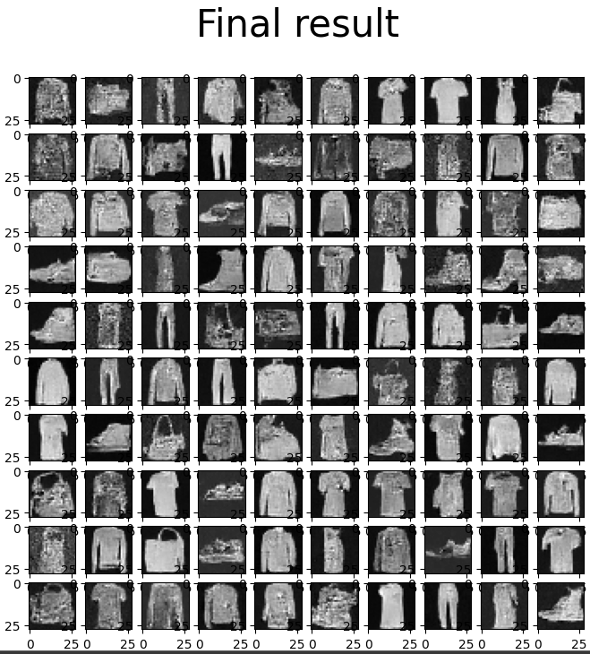
show_images(generated, "Final result")We will try generating new images (100 images), capture the reverse process, and make it into a gif.
from IPython.display import Image

Image(open('fashion.gif' if fashion else 'mnist.gif','rb').read())
The above GIF shows us our network generating 100 images; it starts from pure noise and does a reverse diffusion process; hence, in the end, we get 100 newly generated images based on the learning from our MNIST dataset.
Conclusion
Stable Diffusion’s impressive image generation capabilities result from the intricate interplay of these five key components. The forward and reverse processes work in tandem to learn the relationship between clean and noisy images. The noise schedule optimizes the addition and removal of noise, while positional encoding provides crucial temporal information. Finally, the neural network architecture combines everything, learning to generate high-quality images from noise or text descriptions.
As research advances, we can expect further refinements in each component, potentially leading to more impressive image-generation capabilities. The future of AI-generated art and content looks brighter than ever, thanks to the solid foundation laid by Stable Diffusion and its key components.
If you want to master stable diffusion, checkout our exclusive GenAI Pinnacle Program today!
Frequently Asked Questions
Q1. What is the main difference between Stable Diffusion’s forward and reverse processes?
Ans. The forward process gradually adds noise to an image, while the reverse process removes noise to generate a high-quality image.
Q2. Why is the noise schedule important in Stable Diffusion?
Ans. The noise schedule determines how noise is added and removed, significantly impacting the model’s performance and the quality of generated images.
Q3. What is the purpose of positional encoding in Stable Diffusion?
Ans. Positional encoding helps the model understand the current noise level and stage of the diffusion process, providing a unique representation for each timestep.
Q4. Which neural network architectures are commonly used in Stable Diffusion?
Ans. U-Net and Transformer architectures are commonly used as the backbone for Stable Diffusion models.
Q5. How does the reverse diffusion process generate images?
Ans. The reverse diffusion process iteratively removes noise from a noisy input, gradually reconstructing a high-quality image through multiple denoising steps.
Data science Trainee at Analytics Vidhya, specializing in ML, DL and Gen AI. Dedicated to sharing insights through articles on these subjects. Eager to learn and contribute to the field's advancements. Passionate about leveraging data to solve complex problems and drive innovation.