Introduction
In the current data-focused society, high-dimensional data vectors are now more important than ever for various uses like recommendation systems, image recognition, NLP, and anomaly detection. Efficiently searching through these vectors at scale can be difficult, especially with datasets containing millions or billions of vectors. More advanced indexing techniques are needed as traditional methods like B-trees and hash tables are inadequate for these situations.
Vector databases, designed for handling and searching vectors, have gained popularity due to their rapid search speed, which stems from the indexing methods they use. This blog will deep dive into advanced vector indexing methods that power these databases and ensure blazing-fast searches, even in high-dimensional spaces.
Learning Objectives
- Learn the importance of vector indexing in high-dimensional search.
- Learn the main methods of indexing for effective searches, such as Product Quantization (PQ), Approximate Nearest Neighbor Search (ANNS), and HNSW (Hierarchical Navigable Small World graphs).
- Learn how to implement these indexing techniques with Python-based libraries like FAISS.
- Explore the optimization strategies to ensure efficient querying and retrieval at scale.
This article was published as a part of the Data Science Blogathon.
Table of contents
Challenges of High-Dimensional Vector Search
Searching for the closest neighbors to a query vector in vector search involves measuring “Closeness” using metrics like Euclidean distance, cosine similarity, or other distance metrics. Brute-force methods become more computationally expensive as the data dimensionality increases, often needing linear time complexity, which is O(n), with n representing the number of vectors.
The infamous curse of dimensionality worsens performance by making distance metrics less meaningful, adding further overhead to querying. This necessitates the need for specialized vector indexing mechanisms.
Advanced Indexing Techniques
Effective indexing reduces the search space by creating structures that allow faster retrieval. Key techniques include:
Product Quantization (PQ)
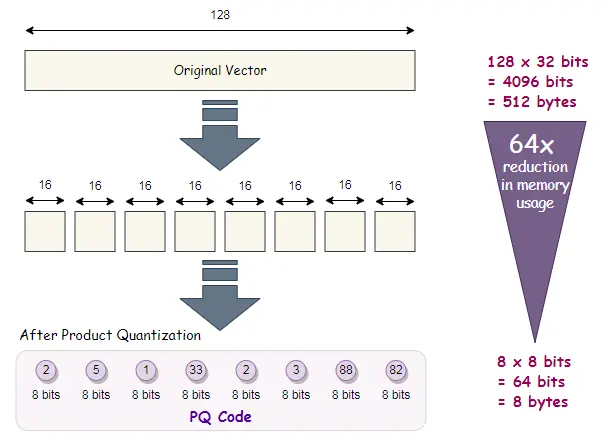
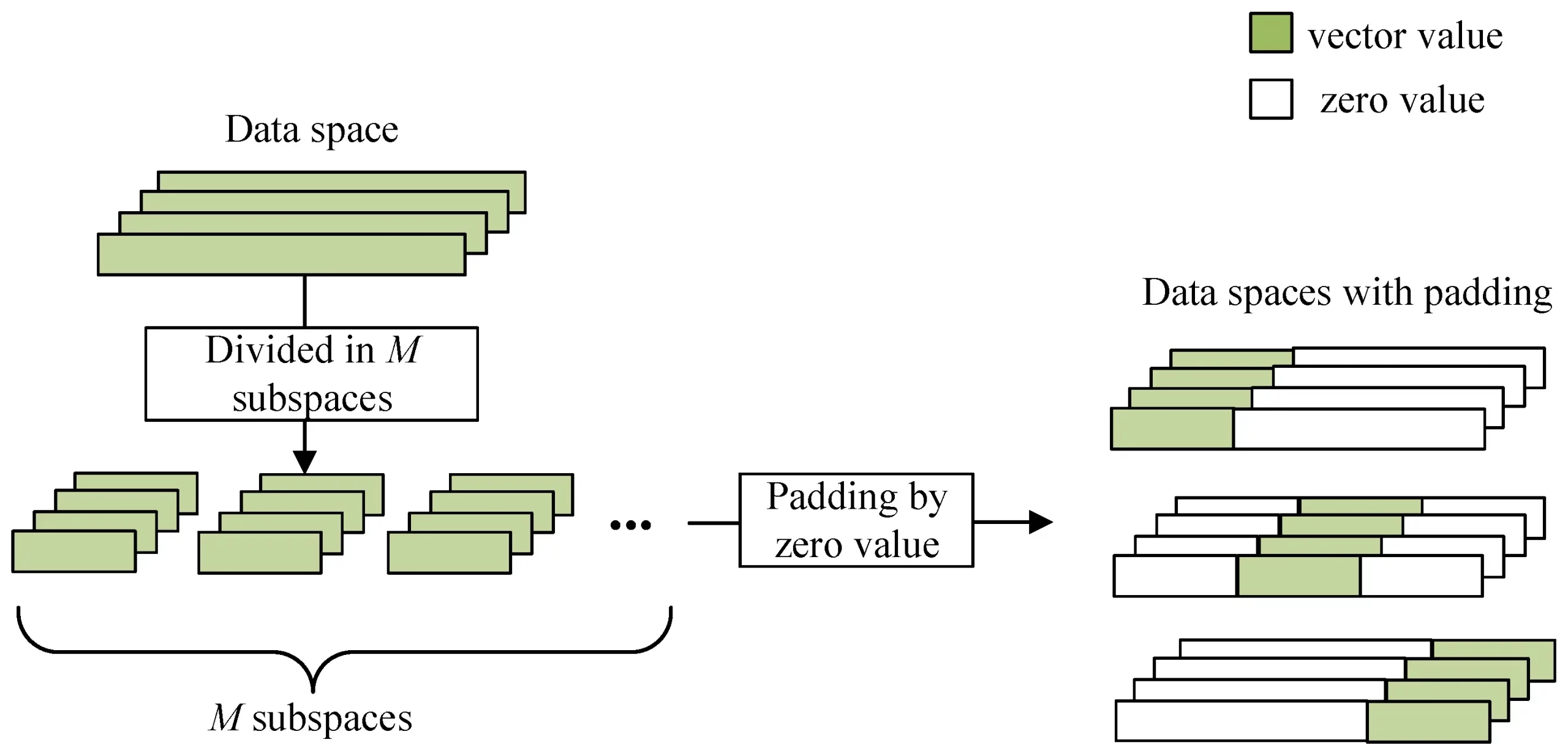
Product Quantization (PQ) is an advanced technique that compresses high-dimensional vectors by partitioning them into subspaces and quantizing each subspace independently. This allows us to enhance the speed of similarity search tasks and greatly decrease the amount of memory needed.

How PQ Works?
- Splitting the Vector: The vector is split into m smaller subvectors.
- Quantization: Each subvector is quantized independently using a small codebook (set of centroids).
- Compressed Representation: The resulting compressed representation is a combination of the quantized subvectors, allowing for efficient storage and search.
Implementing PQ with FAISS
import numpy as np
import faiss
# Create a random set of vectors (size: 10000 vectors of 128 dimensions)
dimension = 128
n_vectors = 10000
data = np.random.random((n_vectors, dimension)).astype('float32')
# Create a product quantizer index in FAISS
quantizer = faiss.IndexFlatL2(dimension)  # L2 distance quantizer
index = faiss.IndexIVFPQ(quantizer, dimension, 100, 8, 8)  # PQ index with 8 sub-vectors

# Train the index with your data
index.train(data)
# Add vectors to the index
index.add(data)
# Perform a search for the closest neighbors
query_vector = np.random.random((1, dimension)).astype('float32')
distances, indices = index.search(query_vector, 5)
print(f"Nearest neighbors (indices): {indices}")
print(f"Distances: {distances}")Output:

In this code, we harness FAISS, a library created by Facebook AI Research, to carry out product quantization. We first create a random set of vectors, train the index, and then use it for vector search.
Advantages of PQ
- Memory Efficiency: PQ dramatically reduces memory usage by compressing vectors.
- Speed: Searches over compressed data are faster than operating on full vectors.
Approximate Nearest Neighbor Search (ANNS)
ANNS offers a method to locate vectors that are “approximately” closest to a query vector, sacrificing some precision for a considerable increase in velocity. The two most commonly used ANNS methods are LSH (Locality Sensitive Hashing) and IVF (Inverted File Index).
Inverted File Index (IVF)
IVF divides the vector space into several partitions (or clusters). Instead of searching the entire dataset, the search is restricted to vectors that fall within a few relevant clusters.
Implementing IVF with FAISS
# Same dataset as above
quantizer = faiss.IndexFlatL2(dimension)
index_ivf = faiss.IndexIVFFlat(quantizer, dimension, 100)  # 100 clusters

# Train the index
index_ivf.train(data)
# Add vectors to the index
index_ivf.add(data)
# Perform the search
index_ivf.nprobe = 10  # Search 10 clusters
distances, indices = index_ivf.search(query_vector, 5)
print(f"Nearest neighbors (indices): {indices}")
print(f"Distances: {distances}")Output:

In this code, we created an Inverted File Index and restricted the search to a limited number of clusters (controlled by the parameter nprobe).

Advantages of ANNS
- Sub-linear Search Time: By restricting the search space, ANNS methods can achieve near-constant search time, making it feasible to handle very large datasets.
- Customizable Trade-off: ANSS methods provide the custom trade-off to fine-tune parameters like nprobe in FAISS to balance between speed and search accuracy.
Hierarchical Navigable Small World (HNSW)
HNSW is a graph-based method where vectors are inserted into a graph, connecting each node to its nearest neighbors. The exploration occurs by moving greedily through the graph from a randomly chosen node. We have:
- Multi-Layer Graph: The graph consists of multiple layers. To allow a fast navigational search, the lower layers are densely connected while the top layers are sparsely connected.
- Greedy Search: The search begins from the topmost layer and progressively moves down, narrowing down to the nearest neighbors.

Implementing HNSW with FAISS
# HNSW index in FAISS
index_hnsw = faiss.IndexHNSWFlat(dimension, 32)  # 32 is the connectivity parameter
# Add vectors to the index
index_hnsw.add(data)
# Perform the search
distances, indices = index_hnsw.search(query_vector, 5)
print(f"Nearest neighbors (indices): {indices}")
print(f"Distances: {distances}")
Output

HNSW has been demonstrated to deliver top-notch performance in terms of search speed while also maintaining high recall rates.
Advantages of HNSW
- Highly Efficient for Large Datasets: It provides logarithmic scaling in search time with respect to the dataset size.
- Dynamic Updates: New vectors can be added efficiently without retraining the entire index.
Optimizing Vector Indexes for Real-World Performance
Let us now on how to optimize vector indexes for real-world performance.
Distance Metrics
The selection of the distance measurement (like Euclidean, cosine similarity) greatly affects the outcome. Researchers commonly use cosine similarity for text embeddings, while they often rely on Euclidean distance for image and audio vectors.
Tuning Index Parameters
Each indexing method has its tunable parameters. For instance:
- nprobe for IVF.
- Sub-vector size for PQ.
- Connectivity for HNSW.
Proper tuning of these parameters is essential to balance the trade-off between speed and recall.
Conclusion
Mastering vector indexing is essential for building high-performance search systems. While brute-force search over large datasets is inefficient, advanced techniques like Product Quantization, Approximate Nearest Neighbor Search, and HNSW enable ultra-fast retrievals without compromising accuracy. By leveraging tools like FAISS and fine-tuning index parameters, developers can create scalable systems capable of handling millions of vectors.
Key Takeaways
- Vector indexing drastically reduces search time, making vector databases highly efficient.
- Product Quantization compresses vectors for faster retrieval, while ANNS and HNSW optimize search by restricting the search space.
- Vector databases are scalable and flexible, making them applicable to various industries, from e-commerce and recommendation systems to image retrieval, NLP, and anomaly detection. The correct choice of vector index can lead to performance improvement for specific use cases.
Frequently Asked Questions
A. Brute-force search compares the query vector against all vectors, whereas approximate nearest neighbor (ANN) search narrows down the search space to a small subset, providing faster results with a slight loss in accuracy.
A. The key metrics for the performance evaluation of a vector database include Recall, Query Latency, Throughput, Index Build Time, and Memory Usage. These metrics help in assessing the balance between speed, accuracy, and resource usage
A. Yes, certain vector indexing methods like HNSW suit dynamic datasets well, enabling efficient insertion of new vectors without requiring retraining of the entire index. However, some techniques, like Product Quantization, may require re-training when large portions of the dataset change.
The media shown in this article is not owned by Analytics Vidhya and is used at the Author’s discretion.


