Dijkstra Algorithm in Python

Introduction

Suppose you are over a map of roads, and you want to know how to get from one city to another using the fewest possible roads. When delivering products through city roads or searching for the most effective route in a network or other systems, the shortest route is crucial. However, one of the best algorithms used in solving them is the Dijkstra’s Algorithm. Also originally thought by Edsger W. Dijkstra in year 1956, this algorithm effectively finds all shortest paths in a weighted graph in which each arc comes with a non negative weight. Here in this tutorial, we will show you how to implement Dijkstra’s Algorithm in steps and for practical use in Python.

Learning Outcomes

• Understand the principles behind Dijkstra’s Algorithm.
• Be able to implement Dijkstra’s Algorithm in Python.
• Learn how to handle weighted graphs and calculate the shortest paths between nodes.
• Know how to optimize and tweak the algorithm for performance in Python.
• Gain hands-on experience by solving a real-world shortest path problem using Python.

What is Dijkstra’s Algorithm?

The algorithm is a greedy algorithm that helps identify the shortest path on a graph that starts with one node. Specifically, in the case of the non-negative weight of edges, the algorithm demonstrates a low complexity. A key idea is to have a pool of nodes for which there exists a best known distance from the source and the expansion to the set of nodes is done by choosing a node with the least known distance. This process continues until and all nodes have been processed.

Here’s a basic breakdown of the algorithm:

• Assign a tentative distance value to every node: set it to 0 for the initial node and to infinity for all others.
• Set the initial node as current and mark all other nodes as unvisited.
• For the current node, check all its unvisited neighbors and calculate their tentative distances through the current node. If this distance is less than the previously recorded tentative distance, update the distance.
• Once done with the neighbors, mark the current node as visited. A visited node will not be checked again.
• Select the unvisited node with the smallest tentative distance as the new current node and repeat steps 3-4.
• Continue the process until all nodes are visited or the shortest distance to the target node is found.

Key Concepts Behind Dijkstra’s Algorithm

Before diving into the implementation, it’s essential to understand some key concepts:

• Graph Representation: The algorithm expects the graph to be done using nodes and edges. Every edge comes with weight – the meaning of which is the distance or cost estimated between two nodes.
• Priority Queue: The ground algorithm that Dijkstra’s Algorithm can employ is the priority queue that determines the next node in the shortest distance.
• Greedy Approach: The algorithm enlarges the shortest known space by yielding the nearest neutral node with respect to a focused node.

How to Implement Dijkstra Algorithm?

We will now implement the Dijkstra algorithm step by step using Python. We’ll represent the graph as a dictionary where keys are nodes and values are lists of tuples representing the adjacent nodes and their corresponding weights.

Step1: Initialize the Graph

We need to represent the graph we are working with. We’ll use a dictionary where the keys are the nodes, and the values are lists of tuples representing the adjacent nodes and their corresponding weights.

graph = {
    'A': [('B', 1), ('C', 4)],
    'B': [('A', 1), ('C', 2), ('D', 5)],
    'C': [('A', 4), ('B', 2), ('D', 1)],
    'D': [('B', 5), ('C', 1)]
}

This graph represents a network where:

• Node A connects to B with weight 1 and to C with weight 4.
• Node B connects to A, C, and D, and so on.

Step 2: Define the Algorithm

Next, we will define the Dijkstra algorithm itself. This function will take the graph and a starting node as input and return the shortest distances from the start node to every other node in the graph. We will use Python’s heapq to implement a priority queue to always explore the node with the smallest known distance first.

import heapq

def dijkstra(graph, start):
    # Initialize distances from the start node to infinity for all nodes except the start node
    distances = {node: float('infinity') for node in graph}
    distances[start] = 0
    # Priority queue to store nodes for exploration
    pq = [(0, start)]  # (distance, node)

    while pq:
        current_distance, current_node = heapq.heappop(pq)

        # Skip this node if it has already been processed with a shorter distance
        if current_distance > distances[current_node]:
            continue

        # Explore neighbors
        for neighbor, weight in graph[current_node]:
            distance = current_distance + weight

            # Only consider this path if it's better than the previously known one
            if distance < distances[neighbor]:
                distances[neighbor] = distance
                heapq.heappush(pq, (distance, neighbor))

    return distances

Step 3: Run the Algorithm

With the algorithm defined, we can now run it on our graph. Here, we’ll specify a starting node (in this case, ‘A’) and call the function to find the shortest paths from ‘A’ to all other nodes.

start_node = 'A'
shortest_paths = dijkstra(graph, start_node)
print(f"Shortest paths from {start_node}: {shortest_paths}")

The output would show the shortest path from node A to all other nodes.

Step 4: Understanding the Output

After running the code, the output will display the shortest paths from the start node (A) to all other nodes in the graph.

If we run the code above, the output will be:

Shortest paths from A: {'A': 0, 'B': 1, 'C': 3, 'D': 4}

This result tells us that:

• The shortest path from A to B is 1.
• The shortest path from A to C is 3.
• The shortest path from A to D is 4.

Example of Dijkstra’s Algorithm

Below we will see the example of Dijkstra’s Algorithm in detail:

Explanation of the Process

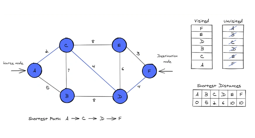
• The algorithm starts at the source node A and calculates the shortest path to all other nodes by evaluating the edge weights between connected nodes.
• Visited and unvisited nodes: Dijkstra’s Algorithm uses two sets of nodes – visited and unvisited. Initially, only the source node (A) is marked as visited, and the rest are considered unvisited. As the algorithm progresses, it visits nodes in order of increasing shortest distance.
• Shortest Distances: The shortest distances are continually updated as the algorithm evaluates all possible paths. Each node is assigned a distance value, starting with 0 for the source node and infinity for the others. As better paths are found, the distances are updated.

Steps Involved

• Starting from node A, the algorithm checks its neighbors and calculates the tentative distances to them. The neighbors are B and C, with distances of 7 and 5, respectively.
• The algorithm chooses node C (distance 5) as the next node to visit since it has the smallest distance.
• From node C, the algorithm evaluates the neighboring nodes D and E, updating their distances.
• The shortest path to node D is found, so the algorithm moves to node D.
• From node D, it evaluates the path to the final node, F.
• After visiting all relevant nodes, the shortest path to node F is determined to be 10.

Final Output

The shortest path from A to F is A → C → D → F, with a total distance of 10.

Shortest Distances

The shortest distance to each node from the source node A is:

• A → A: 0
• A → B: 7
• A → C: 5
• A → D: 6
• A → E: 10
• A → F: 10

The algorithm efficiently calculated the shortest path using the principle of visiting the nearest unvisited node and updating distances based on the edges connecting them.

Enhancements to Dijkstra’s Algorithm

Dijkstra’s Algorithm can be enhanced in various ways to improve its performance, especially for large or specific applications. Below are some key optimizations:

Early Stopping for Targeted Searches

If what you want is simply the shortest path from the source node to the destination node then you can employ early stopping. After reaching the target node it can be stopped because then extra nodes can be overlooked and have less play in this particular algorithm.

Bidirectional Dijkstra’s Algorithm

By running Dijkstra’s Algorithm from both the start and target nodes simultaneously, bidirectional Dijkstra reduces the search space. The two searches meet in the middle, significantly speeding up the process in large graphs.

Optimizing Graph Representation

For sparse graphs, using an adjacency list saves memory and speeds up the algorithm. In dense graphs, an adjacency matrix can be more efficient for edge lookups. Choosing the right graph representation can have a significant impact on performance.

Using a Fibonacci Heap

A Fibonacci heap improves the time complexity of Dijkstra’s Algorithm from O((V + E) log V) to O(E + V log V) by making priority queue operations faster. Though more complex to implement, it’s beneficial for very large graphs with many nodes and edges.

Memory Efficiency in Sparse Graphs

For large, sparse graphs, consider lazy loading parts of the graph or compressing the graph to reduce memory usage. This is useful in applications like road networks or social graphs where memory can become a limiting factor.

Real-World Applications of Dijkstra’s Algorithm

Dijkstra’s Algorithm has numerous applications across various industries due to its efficiency in solving shortest path problems. Below are some key real-world use cases:

GPS and Navigation Systems

Other GPS such as Google Map and Waze, also apply Dijkstra’s Algorithm to determine the shortest path between two destinations. It assists users in finding the best routes depending on roads shared to assist in real-time by providing traffic patterns or congestion, road blockage, or spillage. These systems are further improved by feature enhancements such as early stopping and bidirectional search to find the shortest possible link between two given points.

Network Routing Protocols

Other protocols such as OSPF (Open Shortest Path First) in Computer networking application Dijkstra’s algorithm for analyzing the best possible path for data packet to travel in a network. Data is therefore transmitted with much ease, hence reducing congestion on the linked networks in the system and hence making the overall speed of the system very efficient.

Telecommunications and Internet Infrastructure

Many telecommunication companies apply Dijkstra’s Algorithm in the manner in which the communication’s signal is laid to suit the cables, routers and servers it will pass through. This allows information to be relayed through the shortest and best channels possible and reduce chances of delays and breaks of the channels.

AI and Robotics Pathfinding

In robotics and artificial intelligence conferences, conventions, and applications, Dijkstra’s Algorithm is employed in path-searching techniques which are environments with barriers for robotic or autonomous systems. Since it helps the robots move in the shortest distance while at the same time avoiding object and other obstacles, the algorithm is very essential for applications such as warehousing and automotive where robotic vehicles are now used.

Game Development

Probably the most popular use of Dijkstra’s Algorithm is used in the development of games for path finding in games. Characters as NPCs in games have to move through virtual environment and paths are often optimized and for this Dijkstra helps in giving shortest path among two points and avoids hindrances during game play.

Common Pitfalls and How to Avoid Them

There are some mistakes that are typical for this algorithm and we should beware of them. Below are a few, along with tips on how to avoid them:

Handling Negative Edge Weights

Pitfall: The limitation to this type of algorithm is that it does not recognize negative weights for edges, therefore produces wrong results.

Solution: If your graph contains negative weights then, it is preferable to use algorithms such as Bellman-Ford to solve it, otherwise, normalize all the weights of the graph to be non-negative before using Dijkstra each case.

Inefficient Priority Queue Management

Pitfall: Using an inefficient data structure for the priority queue (like a simple list) can drastically slow down the algorithm, especially for large graphs.

Solution: Always implement the priority queue using a binary heap (e.g., Python’s heapq), or even better, a Fibonacci heap for faster decrease-key operations in large graphs.

Memory Overhead in Large Graphs

Pitfall: Storing large graphs entirely in memory, especially dense graphs, can lead to excessive memory usage, causing performance bottlenecks or crashes.

Solution: Optimize your graph representation based on the type of graph (sparse or dense). For sparse graphs, use an adjacency list; for dense graphs, an adjacency matrix may be more efficient. In very large graphs, consider lazy loading or graph compression techniques.

Ignoring Early Stopping in Specific Searches

Pitfall: Continuing the algorithm after the shortest path to the target node has been found can waste computational resources.

Solution: Implement early stopping by terminating the algorithm as soon as the shortest path to the target node is determined. This is especially important for large graphs or point-to-point searches.

Failing to Choose the Right Algorithm for the Job

Pitfall: Using Dijkstra’s Algorithm in scenarios where a different algorithm might be more suitable, such as graphs with negative weights or cases requiring faster heuristic-based solutions.

Solution: Analyze your graph and the problem context. If negative weights are present, opt for the Bellman-Ford Algorithm. For large graphs where an approximate solution is acceptable, consider using A search* or Greedy algorithms.

Conclusion

Dijkstra’s Algorithm can be described as an effective technique in addressing shortest path problems in cases where weights are non-negative. It is applicable to different areas which include development of networks to games. Following this tutorial, you are now able to perform Dijkstra’s Algorithm in Python by creating and modifying the given code. Altogether this implementation is good to have if one deals with routing problems or would like simply to learn about graph algorithms.

Frequently Asked Questions