Hands-On Multimodal Retrieval and Interpretability (ColQwen + Vespa)

Imagine trying to navigate through hundreds of pages in a dense document filled with tables, charts, and paragraphs. Finding a specific figure or analyzing a trend would be challenging enough for a human; now imagine building a system to do it. Traditional document retrieval systems often rely heavily on text extraction, losing critical context provided by visuals like the layout of tables or balance sheets. What if instead of relying on the traditional approach of OCR + layout detection + chunking + text embedding, we directly just embed the whole page in a document capturing their full visual structure – tables, images, headings, etc. It would be a groundbreaking shift, allowing the system to preserve the rich context within complex documents. ColQwen, an advanced multimodal retrieval model in the ColPali family, does just that.

Learning Objective

1. Understand ColQwen, Multivector Embeddings, and Vespa.
2. Prepare financial PDFs for retrieval by converting pages to images.
3. Embed pages with ColQwen’s Vision Language Model to generate multi-vector embeddings.
4. Configure Vespa with an optimized schema and ranking profile for efficient search.
5. Build a two-phase retrieval pipeline using Vespa’s Hamming distance and MaxSim calculations.
6. Visualize retrieved pages and explore ColQwen’s explainability features for interpretability.

What is ColQwen?

ColQwen is an advanced multimodal retrieval model that uses a Vision Language Model (VLM) approach that processes entire document pages as images. Using multi-vector embeddings it creates a richly layered representation of the page that maintains each page’s structure and context. It is built specifically to simplify and enhance document retrieval, especially for visually dense documents.

Why ColQwen is Different?

Traditional systems break down a document to its basics—OCR extracts the text, then splits, tags, and embeds it. While this approach works for text-only files, it limits the detail retrievable from complex documents where layout matters. In financial reports or research papers, information resides not only in the words but also in their visual structure—how headings, numbers, and summaries are positioned relative to one another.

With ColQwen, the process is simple. Instead of reducing pages to smaller text chunks, ColQwen’s multi-vector embeddings capture the whole page image, preserving both text and visual cues.

What is Multivector embeddings?

💡We have been talking about multi-vector embeddings, but what exactly are multi-vector embeddings, and how are they used here?

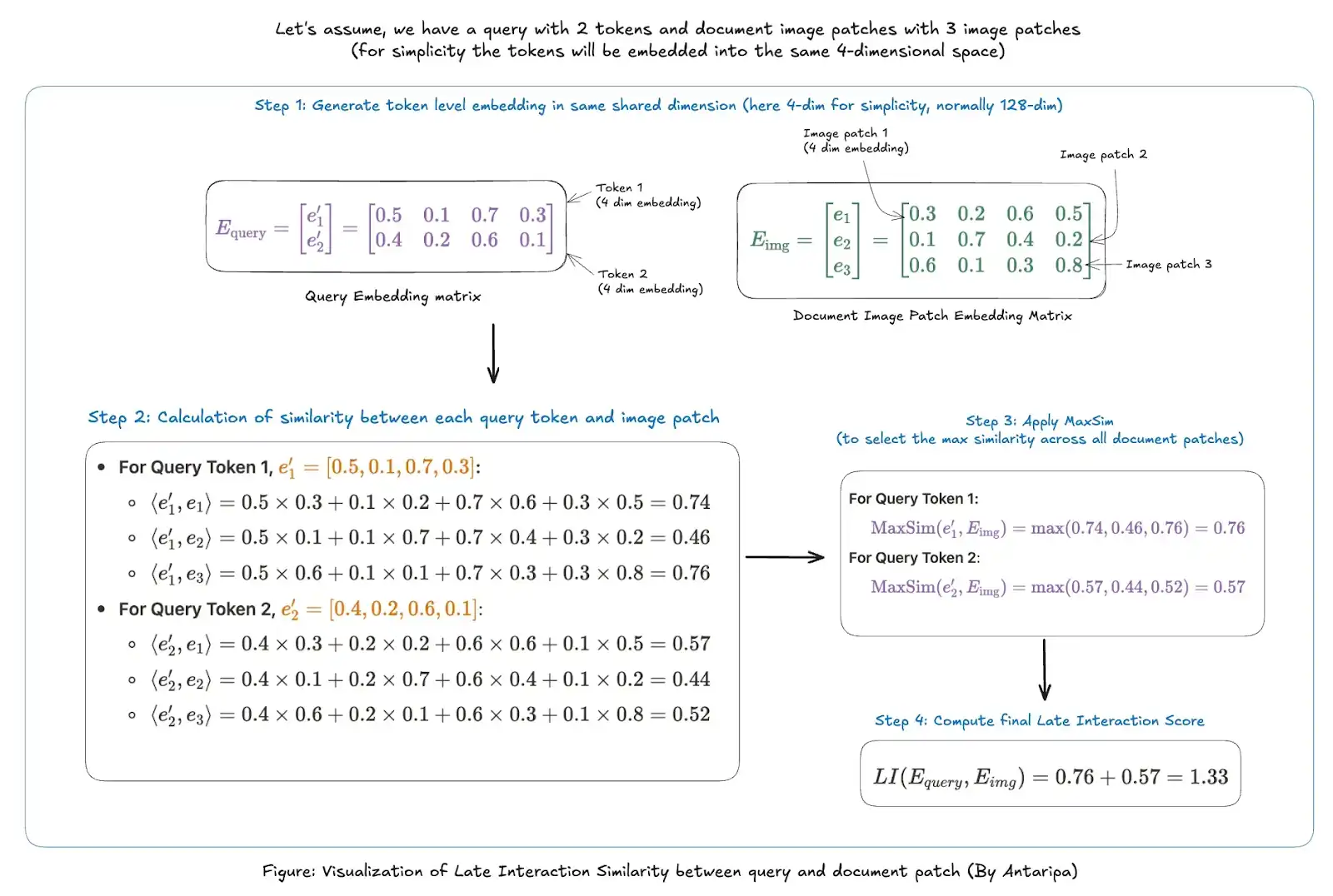
Unlike traditional single-vector embeddings that use a single dense representation for an entire document, multi-vector embeddings create multiple, focused embeddings—one for each query token. Originally developed for models like ColBERT (for text-based retrieval with “late interaction”), multi-vector embeddings ensure that each query token can interact with the most relevant portions of a document.

In ColQwen (and ColPali), this technique is adapted for visually complex documents. Each page image is divided into patches, with each section—whether a table, heading, or figure – receiving its own embedding. When a query is made, each token in the query can search across these patches, surfacing the most relevant visual and textual parts of the page. This way, ColQwen retrieves exactly the right content, which is structured and contextually aware. 

Patches: In ColQwen, images are divided into small sections or “patches.” Each patch has its own embedding, allowing the model to focus on specific areas of an image rather than processing it as a whole. Patches are helpful for breaking down visually complex pages so that each part can be analyzed in detail.

Please check the example below to understand MaxSim and late-interaction better:

ColPali vs ColQwen2: what’s new?

Unlike ColPali, which resizes images and alters aspect ratios, ColQwen2 accepts images in their dynamic resolutions, preserving their original aspect ratios. This is achieved by processing images at their native resolutions, ensuring that the visual content remains unaltered and accurately represented.

In addition, ColQwen2 allows for the adjustment of image resolution, which directly influences the number of visual tokens extracted from the image. By controlling the resolution, users can balance between the storage requirements and retrieval performance. Higher resolutions yield more visual tokens, potentially enhancing retrieval accuracy but increasing storage needs. Conversely, lower resolutions reduce storage demands but may impact retrieval effectiveness. This flexibility enables users to tailor the system to their specific performance and resource constraints.

What is Vespa?

Vespa is an open-source vector database and search platform that handles dense and sparse data. It is one of two vector databases currently supporting multi-vector representations (the other one is QDrant). It enables data retrieval, custom ranking, and indexing strategies.

In this hands-on guide, we’ll pair ColQwen’s visual embedding power with Vespa‘s search platform, to create a robust document retrieval system. Vespa will serve as our vector db query engine. We’ll set up a pipeline to handle complex documents like financial reports, turning visually dense pages into searchable representations and enabling quick, accurate retrieval.

Let’s dive in and get our hands dirty!

Colab notebook:  ColQwen_pdf_retrieval_and_interpretability.ipynb

NOTE: I have used both the A100 40GB GPU (colab pro) and the T4 GPU, which comes with free colab; both will work. Just that you will be able to embed very few document pages with the free version (OOM issues will show up).

Step 1: Installation

# Install essential libraries
!pip install transformers --upgrade
!pip install colpali-engine --upgrade
!apt-get install poppler-utils  # for handling PDF images
!pip install pdf2image pypdf
!pip install qwen_vl_utils
!pip install pyvespa vespacli  # Vespa tools

Note: Make sure you have poppler-utils installed, as it’s needed to convert PDF pages into images.

Step 2: Setting Up ColQwen for Image Embedding

First, we import ColQwen, a model from the ColPali family, which uses a Vision Language Model (VLM) approach to process entire PDF pages as images.

from colpali_engine.models import ColQwen2, ColQwen2Processor

# Initialize ColQwen model and processor
model = ColQwen2.from_pretrained(
    "vidore/colqwen2-v0.1",
    torch_dtype=torch.bfloat16,  # Use float16 if GPU does not support bfloat16
    device_map="auto",
)
processor = ColQwen2Processor.from_pretrained("vidore/colqwen2-v0.1")
model = model.eval()

Step 3: Preparing the PDFs

Here, we’ll load and preprocess two sample PDFs. You can customize the URLs to use different documents. Both pdfs are finance documents, the second one has a more complex structure (tables and data are embedded in the image). Both of these pdfs have 35 pages each.

pdf_lists = [

    {"header": "Tesla finance",
    "Url": "<https://ir.tesla.com/_flysystem/s3/sec/000162828024043432/tsla-20241023-gen.pdf>"},
   
    {"header": "Understanding company finance",
    "url": "<https://www.pwc.com/jm/en/research-publications/pdf/basic-understanding-of-a-companys-financials.pdf>"}
   
]

Step 4: Downloading and Processing PDF Pages as Images

Create helper functions to download PDFs and convert each page into images for embedding.

import requests
from io import BytesIO
from pdf2image import convert_from_path

# Utility to download a PDF file from a URL
def download_pdf(url):
    response = requests.get(url)
    if response.status_code == 200:
        return BytesIO(response.content)
    else:
        raise Exception("Failed to download PDF")

# Convert PDF pages to images
def get_pdf_images(pdf_url):
    pdf_file = download_pdf(pdf_url)
    pdf_file.seek(0)
    temp_file_path = "temp.pdf"
    with open(temp_file_path, "wb") as f:
        f.write(pdf_file.read())
    return convert_from_path(temp_file_path)

download_pdf fetches the PDF from the URL, while get_pdf_images saves and converts each page to an image format compatible with ColQwen.

Step 5: Encoding and Generating Embeddings for PDF Pages

Now, we’ll use ColQwen to create multi-vector embeddings for each page image. We batch-process images to generate embeddings efficiently. Each PDF is now represented by embeddings for each page image, preserving both text and layout.

from torch.utils.data import DataLoader
from tqdm import tqdm

# Generate embeddings for images using ColQwen
def generate_image_embeddings(images, model, processor, batch_size=4):  # modify batch_size according to your machine's capability
    embeddings = []
    dataloader = DataLoader(images, batch_size=batch_size, shuffle=False,
                            collate_fn=lambda x: processor.process_images(x))
    for batch in tqdm(dataloader):
        with torch.no_grad():
            batch = {k: v.to(model.device) for k, v in batch.items()}
            batch_embeddings = model(**batch).to("cpu")
            embeddings.extend(list(batch_embeddings))
    return embeddings
   

# Process and store embeddings for each PDF in the list
for pdf in pdf_lists:
    header = pdf.get("header", "Unnamed Document")
    print(f"Processing {header}")
    try:
        pdf_page_images = get_pdf_images(pdf["url"])
        pdf["images"] = pdf_page_images
        pdf_embeddings = generate_image_embeddings(pdf_page_images, model, processor)
        pdf["embeddings"] = pdf_embeddings
    except Exception as e:
        print(f"Error processing {header}: {e}")

Output

Process for Tesla finance pdf started

100%|██████████| 9/9 [00:41<00:00,  4.61s/it]

Process for Basic understanding of company finance pdf started

100%|██████████| 9/9 [00:39<00:00,  4.40s/it]

Step 6: Encoding Images as Base64 and Structuring Data for Vespa

Utility function here for encoding of images in base64 format and resizing the image in a presentable format.

import base64
from PIL import Image

# Encode images in base64
def encode_images_base64(images):
    base64_images = []
    for image in images:
        buffered = BytesIO()
        image.save(buffered, format="JPEG")
        base64_images.append(base64.b64encode(buffered.getvalue()).decode('utf-8'))
    return base64_images
   
   
def resize_image(images, max_height=800):
    resized_images = []
    for image in images:
        width, height = image.size
        if height > max_height:
            ratio = max_height / height
            new_width = int(width * ratio)
            new_height = int(height * ratio)
            resized_images.append(image.resize((new_width, new_height)))
        else:
            resized_images.append(image)
    return resized_images

Why Base64?

The Base64 encoding is necessary for storing image data in Vespa’s raw field format.

Now, prepare the data that will be inserted into Vespa vector database. The multivector embeddings for the images were already generated above. Here, we are doing slight modification -> binary quantization of vectors (i.e., float values will be converted to 0, 1), and images are converted to base64 encoding for easily storing the encoded string of the image to Vespa.

Binary quantization: Say we have a vector [0.8, -0.5, 1.2, 0.3], upon binary quantization the vector is transformed to [1, 0, 1, 1]. Values less than equal to zero get transformed to 0, and more than 0 get transformed to 1.

vespa_feed = []
for pdf in pdf_lists:
    url = pdf["url"]
    title = pdf["header"]
    base64_images = encode_images_base64(resize_image(pdf["images"]))

    for page_number, (embedding, image, base64_img) in enumerate(zip(pdf["embeddings"], pdf["images"], base64_images)):
        embedding_dict = dict()
        for idx, patch_embedding in enumerate(embedding):
            binary_vector = (
                np.packbits(np.where(patch_embedding > 0, 1, 0))
                .astype(np.int8)
                .tobytes()
                .hex()
            )
            embedding_dict[idx] = binary_vector
        page = {
            "id": hash(url + str(page_number)),
            "url": url,
            "title": title,
            "page_number": page_number,
            "image": base64_img,
            "embedding": embedding_dict,
        }
        vespa_feed.append(page)

This process stores each document’s metadata, embeddings, and images in a format compatible with Vespa. The embeddings are binarized using np.packbits, allowing for faster and memory-efficient hamming distance calculations.

# Verifying the output of data once
print("Total documents in vespa_feed: ", len(vespa_feed))   # total numbers pages -> including all pdfs
print(vespa_feed[0].keys())

Output

Total documents in vespa_feed: 70

dict_keys(['id', 'url', 'title', 'page_number', 'image', 'embedding'])

Binary Quantization

Binary quantization converts high-dimensional vectors (real-valued embeddings) into binary codes (e.g., 001101). This involves encoding each element as either 1 or 0, reducing the memory footprint of embeddings, and enabling rapid similarity computation. By binarizing embeddings, Vespa claimed to have reduced the storage size by about 32x compared to using float32 vectors.

💡Binary Vector: A binary vector is a simplified representation of data, where each element is either 0 or 1.

For binary quantized vectors, similarity can be measured using Hamming distance. The Hamming distance between two binary vectors simply counts the mismatches of bits (0 vs 1). A smaller Hamming distance means the vectors are more similar. 

For example: Let there be two vectors, Vector A: [1, 0, 1, 1], Vector B: [1, 1, 1, 0]
Hamming Distance between them: 2 (bits differ at positions 2 and 4)

In contrast to cosine similarity, Hamming distance is computationally inexpensive due to its reliance on bitwise operations like XOR.

Benefits of Binary Quantization:

• Storage Efficiency: Binary vectors use fewer bits, requiring significantly less memory.
• Speed: Binary vectors enable fast similarity computation through Hamming distance, which uses bitwise operations.

While binarization may slightly reduce accuracy, it significantly boosts speed, making it ideal for high-speed retrieval in large document sets.

💡Why cosine similarity can’t be used with binary vectors? In binary vectors, each dimension is either 0 or 1, so there isn’t a concept of “magnitude” as we have in continuous real-valued vectors. Whereas, to calculate cosine similarity, it’s dependent on real-valued vectors with magnitudes so that it can measure the cosine of the angle between two vectors.

Not going in-detail for binary quantization, this resource covers brilliantly: Scaling ColPali to billions of PDFs with Vespa

Visualization of Binary Quantization of vectors and Hamming Distance calculation:

Step 7: Creating a Vespa Schema

We define the Vespa schema including fields, data types, indexing, and the fields that will be available for search matching. Both documents and metadata are defined here. This is pretty common in every database to define a schema before inserting data (like elastic search, weaviate, etc).

from vespa.package import ApplicationPackage, Schema, Document, Field, HNSW

colpali_schema = Schema(
    name="finance_data_schema",  # can name this anything
    document=Document(
        fields=[
            Field(name="id", type="string", indexing=["summary", "index"]),
            Field(name="url", type="string", indexing=["summary", "index"]),
            Field(name="title", type="string", indexing=["summary", "index"], index="enable-bm25"),
            Field(name="page_number", type="int", indexing=["summary", "attribute"]),
            Field(name="image", type="raw", indexing=["summary"]),
            Field(name="embedding", type="tensor<int8>(patch{}, v[16])", indexing=["attribute", "index"],
                  ann=HNSW(distance_metric="hamming"))
        ]
    )
)

The HNSW (Hierarchical Navigable Small World) index enables efficient similarity searches on vector embeddings.

Step 8: Defining Query Tensors for Retrieval

To process complex queries, we define multiple query tensors that allow Vespa to use both binary and float representations. This setup enables efficient matching using Hamming distance (for quick filtering with binary tensors) and MaxSim (for precise scoring with float tensors).

input_query_tensors = []
MAX_QUERY_TERMS = 64
for i in range(MAX_QUERY_TERMS):
    input_query_tensors.append((f"query(rq{i})", "tensor<int8>(v[16])"))

input_query_tensors.append(("query(qt)", "tensor<float>(querytoken{}, v[128])"))
input_query_tensors.append(("query(qtb)", "tensor<int8>(querytoken{}, v[16])"))

• Binary Tensors (tensor<int8>(v[16])): Each query term is represented as a binary tensor (e.g., query(rq{i})), used for fast initial filtering.
• Float Tensors (tensor<float>(querytoken{}, v[128])): Each query term also has a float tensor (query(qt)), allowing for detailed similarity scoring during re-ranking.

This combination of tensor types lets Vespa focus on relevant document sections and ensures high precision in retrieval, even for visually complex queries.

Step 9: Creating a Multi-Phase Ranking Profile in Vespa

Next, we define a ranking profile in Vespa that uses both Hamming distance (for binary similarity) and MaxSim (for float-based late interaction similarity) to rank documents. This profile enables a two-phase ranking: a first phase for initial filtering using binary similarity, and a second phase for re-ranking with continuous (float) similarity scores.

from vespa.package import RankProfile, Function, FirstPhaseRanking, SecondPhaseRanking

colpali_retrieval_profile = RankProfile(
    name="retrieval-and-rerank",
    inputs=input_query_tensors,
    functions=[
        # First phase: Binary similarity using Hamming distance for fast filtering
        Function(
            name="max_sim_binary",
            expression="""
                sum(
                  reduce(
                    1/(1 + sum(
                        hamming(query(qtb), attribute(embedding)) ,v)
                    ),
                    max,
                    patch
                  ),
                  querytoken
                )
            """,
        ),
        # Second phase: Float-based similarity using MaxSim for refined re-ranking
        Function(
            name="max_sim",
            expression="""
                sum(
                    reduce(
                        sum(
                            query(qt) * unpack_bits(attribute(embedding)) , v
                        ),
                        max, patch
                    ),
                    querytoken
                )
            """,
        )
    ],
    first_phase=FirstPhaseRanking(expression="max_sim_binary"),   # Initial filtering with binary similarity
    second_phase=SecondPhaseRanking(expression="max_sim", rerank_count=10),  # Reranking top 10 results with float similarity
)
colpali_schema.add_rank_profile(colpali_retrieval_profile)

Why Two-phase Ranking – MaxSim and Hamming Distance

When dealing with massive datasets in vector databases like Vespa, we need a way to find relevant entries quickly. In ColQwen’s approach, we use Hamming Distance and MaxSim functions to handle this task efficiently. Here’s how each function contributes:

• Hamming Distance: This is a fast, initial filter that works with binary vectors (simplified versions of the embeddings). It compares vectors in terms of bitwise similarity and calculates the number of bits that differ between the query and each document. Hamming Distance is computationally lightweight, making it a great choice for quick filtering in the initial phase. By reducing the number of candidates at this stage, we ensure that only the most likely matches move on to the next round of ranking. Here, The max_sim_binary function calculates binary similarity between query(qtb) and attribute(embedding) by counting bitwise matches.
  
• MaxSim: This function is used for a more precise comparison. MaxSim directly compares embeddings in a continuous vector space, capturing subtle differences that the binary filter might overlook. The max_sim function multiplies each query token (query(qt)) with corresponding document patches and sums the maximum similarity scores across patches.

Binary Vector: A binary vector is a simplified representation of data, where each element is either 0 or 1. This simplification makes certain calculations faster, especially when using Hamming Distance, which is based on comparing differences between bits.

Step 10: Deploying Vespa Application

With the configured application, we can now deploy the Vespa schema and application to Vespa Cloud.

To deploy the application to Vespa Cloud we need to create an account (free trial works) and then a tenant in the Vespa cloud.

For this step, tenant_name and app_name are required, which you can set up in Vespa Cloud after creating your account. After the tenant is created, create an application in Vespa Cloud and paste the name here below. Since we are not giving the key below, you need to log in interactively from here.

from vespa.deployment import VespaCloud

app_name = "colqwen_retrieval_app" # can name it anything
tenant_name = "your-tenant-name"  # Replace with your Vespa Cloud tenant name
vespa_application_package = ApplicationPackage(name=app_name, schema=[colpali_schema])

vespa_cloud = VespaCloud(tenant=tenant_name, application=app_name, application_package=vespa_application_package)

app: Vespa = vespa_cloud.deploy()

After deployment, make sure to verify the application’s status in the Vespa Cloud Console.

Step 10: Feeding Data to Vespa for Indexing

With our ranking profile set, we can now feed the pre-processed data to Vespa. Each document (or page) is embedded, binarized, and ready to be indexed for retrieval.

from vespa.io import VespaResponse

async with app.asyncio(connections=1, timeout=180) as session:
    for page in vespa_feed:
        response: VespaResponse = await session.feed_data_point(
            data_id=page["id"], fields=page, schema="finance_data_schema"
        )
        if not response.is_successful():
            print(response.json())

Output

100%|██████████| 70/70 [00:51<00:00,  1.36it/s]

A total of 70 pages (from both PDFs) are inserted into Vespa. Each document (page) is uploaded to Vespa along with its ID, URL, title, page number, base64 image, and binary embeddings for retrieval. This setup allows for both metadata-based filtering (like by title) and embedding-based similarity searches.

Step 11: Querying Vespa and Displaying Results

Utility function to display the top retrieved results (images) in presentable format. Since we have saved base64 format image in Vespa, first we need to decode that and then display.

from IPython.display import display, HTML

# Display query results images
def display_query_results(query, response, hits=5):
    query_time = response.json.get("timing", {}).get("searchtime", -1)
    query_time = round(query_time, 2)
    count = response.json.get("root", {}).get("fields", {}).get("totalCount", 0)
    html_content = f"<h3>Query text: '{query}', query time {query_time}s, count={count}, top results:</h3>"

    for i, hit in enumerate(response.hits[:hits]):
        title = hit["fields"]["title"]
        url = hit["fields"]["url"]
        page = hit["fields"]["page_number"]
        image = hit["fields"]["image"]
        score = hit["relevance"]

        html_content += f"<h4>PDF Result {i + 1}</h4>"
        html_content += f'<p><strong>Title:</strong> <a href="{url}">{title}</a>, page {page+1} with score {score:.2f}</p>'
        html_content += (
            f'<img src="data:image/png;base64,{image}" style="max-width:100%;">'
        )

    display(HTML(html_content))

Now, we can query Vespa using ColQwen embeddings and visualize the results. The display_query_results function formats and displays the top results, including image previews and relevance scores for each page.

queries = ["balance at 1 July 2017 for equity holders"]  # you can pass multiple queries here

dataloader = DataLoader(
    queries,
    batch_size=1,
    shuffle=False,
    collate_fn=lambda x: processor.process_queries(x),
)
qs = []
for batch_query in dataloader:
    with torch.no_grad():
        batch_query = {k: v.to(model.device) for k, v in batch_query.items()}
        embeddings_query = model(**batch_query)
        qs.extend(list(torch.unbind(embeddings_query.to("cpu"))))

Generated the embeddings of the query from the same ColQwen model.

Next, we perform the final search on the indexed documents, retrieving pages based on the query tokens and their embeddings, and the display_query_results function shows each page’s title, URL, page number, relevance score, and a preview image.

target_hits_per_query_tensor = (
    5  # this is a hyperparameter that can be tuned for speed versus accuracy
)
async with app.asyncio(connections=1, timeout=180) as session:
    for idx, query in enumerate(queries):
        float_query_embedding = {k: v.tolist() for k, v in enumerate(qs[idx])}
        binary_query_embeddings = dict()
        for k, v in float_query_embedding.items():
            binary_query_embeddings[k] = (
                np.packbits(np.where(np.array(v) > 0, 1, 0)).astype(np.int8).tolist()
            )

        # The mixed tensors used in MaxSim calculations
        # We use both binary and float representations
        query_tensors = {
            "input.query(qtb)": binary_query_embeddings,
            "input.query(qt)": float_query_embedding,
        }
        # The query tensors used in the nearest neighbor calculations
        for i in range(0, len(binary_query_embeddings)):
            query_tensors[f"input.query(rq{i})"] = binary_query_embeddings[i]
        nn = []
        for i in range(0, len(binary_query_embeddings)):
            nn.append(
                f"({{targetHits:{target_hits_per_query_tensor}}}nearestNeighbor(embedding,rq{i}))"
            )
        # We use a OR operator to combine the nearest neighbor operator
        nn = " OR ".join(nn)
        response: VespaQueryResponse = await session.query(
            yql=f"select title, url, image, page_number from pdf_page where {nn}",
            ranking="retrieval-and-rerank",
            timeout=120,
            hits=3,
            body={**query_tensors, "presentation.timing": True},
        )
        assert response.is_successful()
        display_query_results(query, response)

Output

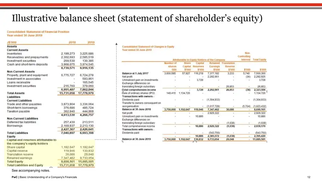
Result 1 for query: “balance at 1 July 2017 for equity holders”, is image 11

Result 2 for query: “balance at 1 July 2017 for equity holders”, is image 5

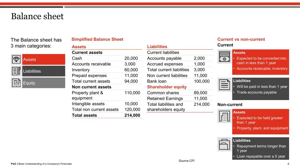
Here, showing the top two retrieved outputs above. As you can see, the top image exactly has the terms “balance”, “1 July 2017”, “equity”.

Now let’s extract the same pdf page from pdfreader to check if the text was present in text format or was embedded in an image. This step is interesting because it shows the limitations of a standard PDF text extractor when dealing with complex documents where text is primarily embedded as images. (Ps: if you open this PDF, you’ll notice that most of the text isn’t selectable.)

By extracting text from the second PDF, we illustrate that the PDF extractor struggles to retrieve meaningful text since almost everything is embedded within images.

url = "<https://www.pwc.com/jm/en/research-publications/pdf/basic-understanding-of-a-companys-financials.pdf>"

pdf_file = download_pdf(pdf["url"])
pdf_file.seek(0)  # Reset file pointer for image conversion

# gets text of each page from the PDF
temp_file_path = "test.pdf"
with open(temp_file_path, "wb") as f:
    f.write(pdf_file.read())
reader = PdfReader(temp_file_path)
page_texts = []
for page_number in range(len(reader.pages)):
    page = reader.pages[page_number]
    text = page.extract_text()
    page_texts.append(text)
   
print(page_texts[11])  # printing the text from 11th index page (from 2nd pdf)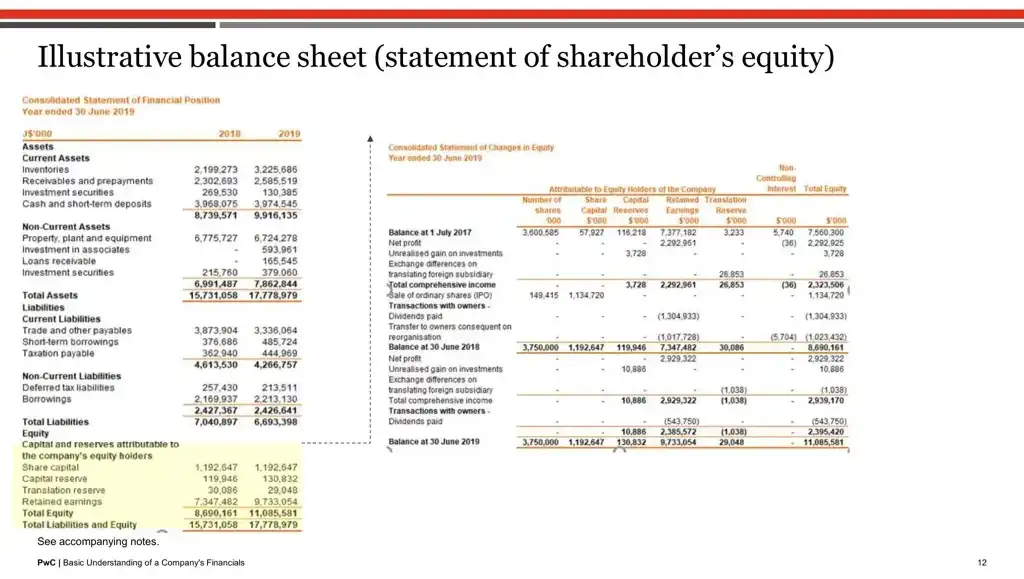

Output

"12 PwC | Basic Understanding of a Company's Financials

Illustrative balance sheet (statement of shareholder’s equity)

See accompanying notes."

As we can see hardly any text could be extracted because of the embedded nature.

Step 12: Interpretability with ColQwen – Visualizing Relevant Patches

A major advantage of ColQwen lies in its interpretability. Beyond simply returning results, ColQwen provides insights into why certain pages or sections of documents were chosen based on the query. This transparency is achieved through similarity maps, which visually highlight the most relevant areas of each retrieved document.

query = "balance at 1 July 2017 for equity holders"
idx = 11 # top retrieved index
top_image = pdf_lists[1]["images"][idx]
pdf_embeddings =  pdf_lists[1]["embeddings"]

# Get the number of image patches
n_patches = processor.get_n_patches(
    image_size=top_image.size,
    patch_size=model.patch_size,
    spatial_merge_size=model.spatial_merge_size,
)

# Get the tensor mask to filter out the embeddings that are not related to the image
image_mask = processor.get_image_mask(processor.process_images([top_image]))

batch_queries = processor.process_queries([query]).to(model.device)
# Generate the similarity maps
batched_similarity_maps = get_similarity_maps_from_embeddings(
    image_embeddings=pdf_embeddings[idx].unsqueeze(0).to("cuda"),
    query_embeddings=model(**batch_queries),
    n_patches=n_patches,
    image_mask=image_mask,
)

query_content = processor.decode(batch_queries.input_ids[0]).replace(processor.tokenizer.pad_token, "")
query_content = query_content.replace(processor.query_augmentation_token, "").strip()
query_tokens = processor.tokenizer.tokenize(query_content)

# Get the similarity map for our (only) input image
similarity_maps = batched_similarity_maps[0]  # (query_length, n_patches_x, n_patches_y)

Above, we’re creating a “similarity map” to interpret how the model connects specific parts of a query (like “balance at 1 July 2017 for equity holders”) to regions of an image extracted from a PDF. This similarity map helps visually represent which parts of the image are relevant to each word in the query, making the model’s decision process interpretable.

print(query_tokens) # check the tokens of the query after tokenization process

Output

['Query', ':', 'Ġbalance', 'Ġat', 'Ġ', '1', 'ĠJuly', 'Ġ', '2', '0', '1', '7', 'Ġfor', 'Ġequity', 'Ġholders']

We will visualize the heatmap for two tokens in the query “balance” and “July”:

idx = 11  # top retrieved page from vespa
top_image = pdf_lists[1]["images"][idx]
token_idx = 2  # visualizing for 2nd index token from the query_tokens which is 'balance'

fig, ax = plot_similarity_map(
    image=top_image,
    similarity_map=similarity_maps[token_idx],
    figsize=(8, 8),
    show_colorbar=False,
)

max_sim_score = similarity_maps[token_idx, :, :].max().item()
ax.set_title(f"Token #{token_idx}: `{query_tokens[token_idx].replace('Ġ', '_')}`. MaxSim score: {max_sim_score:.2f}", fontsize=14)

del query_content, query_tokens, batch_queries, batched_similarity_maps, similarity_maps, image_mask, n_patches, top_image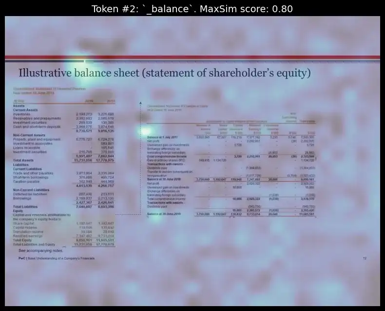

Visualizing the heatmap for the token ‘July’:

idx = 11
top_image = pdf_lists[1]["images"][idx]
token_idx = 6  # visualizing for 2nd index token from the query_tokens which is 'July'

fig, ax = plot_similarity_map(
    image=top_image,
    similarity_map=similarity_maps[token_idx],
    figsize=(8, 8),
    show_colorbar=False,
)

max_sim_score = similarity_maps[token_idx, :, :].max().item()
ax.set_title(f"Token #{token_idx}: `{query_tokens[token_idx].replace('Ġ', '_')}`. MaxSim score: {max_sim_score:.2f}", fontsize=14)

del query_content, query_tokens, batch_queries, batched_similarity_maps, similarity_maps, image_mask, n_patches, top_image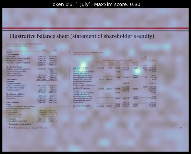

We can see how, for each of the respective tokens, the model could properly figure out the layout position those words were present and highlighted them.

The interpretability layer reveals which parts of the document matched the query, allowing users to understand the retrieval logic better. This feature enhances transparency by revealing why certain pages were selected.

Conclusion

In this blog, we explored how ColQwen’s advanced Vision Language Model, combined with Vespa’s powerful multi-vector search, is reshaping the way we retrieve visually dense document data. By directly embedding entire pages as images and leveraging multi-vector embeddings, this approach avoids the pitfalls of traditional text-only extraction, making it possible to retrieve information that is not only accurate but also contextually aware.

ColQwen’s interpretability and explainability bring much-needed transparency to industries like finance, law, and healthcare, where context is everything.

Advancements in multimodal retrieval have been taking up this year and this powerful combination of ColQwen + Vespa is just one such example of how we can make document search as intuitive and reliable. Hope you liked the blog, let me know if you have any thoughts.

If you are looking for a Generative AI course online then explore: GenAI Pinnacle Program

Frequently Asked Questions

Antaripa Saha

Hi, I'm Antaripa Saha, Machine Learning Engineer II at a US-based startup. I am passionate about math, generative AI, and the latest advancements in VLMs and LLMs. I like deep-diving research papers and breaking them down in my blogs.
My twitter profile: https://twitter.com/doesdatmaksense