How to Evaluate LLMs Using Hugging Face Evaluate

Evaluating large language models (LLMs) is essential. You need to understand how well they perform and ensure they meet your standards. The Hugging Face Evaluate library offers a helpful set of tools for this task. This guide shows you how to use the Evaluate library to assess LLMs with practical code examples.

Understanding the Hugging Face Evaluate Library

The Hugging Face Evaluate library provides tools for different evaluation needs. These tools fall into three main categories:

1. Metrics: These measure a model’s performance by comparing its predictions to ground truth labels. Examples include accuracy, F1-score, BLEU, and ROUGE.
2. Comparisons: These help compare two models, often by examining how their predictions align with each other or with reference labels.
3. Measurements: These tools investigate the properties of datasets themselves, like calculating text complexity or label distributions.

You can access all these evaluation modules using a single function: evaluate.load().

Getting Started

Installation

First, you need to install the library. Open your terminal or command prompt and run:

pip install evaluate

pip install rouge_score # Needed for text generation metrics

pip install evaluate[visualization] # For plotting capabilities

These commands install the core evaluate library, the rouge_score package (required for the ROUGE metric often used in summarization), and optional dependencies for visualization like radar plots.

Loading an Evaluation Module

To use a specific evaluation tool, you load it by name. For instance, to load the accuracy metric:

import evaluate

accuracy_metric = evaluate.load("accuracy")

print("Accuracy metric loaded.")

Output:

This code imports the evaluate library and loads the accuracy metric object. You will use this object to compute accuracy scores.

Basic Evaluation Examples

Let’s walk through some common evaluation scenarios.

Computing Accuracy Directly

You can compute a metric by providing all references (ground truth) and predictions at once.

import evaluate

# Load the accuracy metric

accuracy_metric = evaluate.load("accuracy")

# Sample ground truth and predictions

references = [0, 1, 0, 1]

predictions = [1, 0, 0, 1]

# Compute accuracy

result = accuracy_metric.compute(references=references, predictions=predictions)

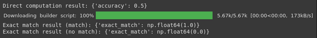
print(f"Direct computation result: {result}")

# Example with exact_match metric

exact_match_metric = evaluate.load('exact_match')

match_result = exact_match_metric.compute(references=['hello world'], predictions=['hello world'])

no_match_result = exact_match_metric.compute(references=['hello'], predictions=['hell'])

print(f"Exact match result (match): {match_result}")

print(f"Exact match result (no match): {no_match_result}")

Output:

Explanation:

1. We define two lists: references holds the correct labels, and predictions holds the model’s outputs.
2. The compute method takes these lists and calculates the accuracy, returning the result as a dictionary.
3. We also show the exact_match metric, which checks if the prediction perfectly matches the reference.

Incremental Evaluation (Using add_batch)

For large datasets, processing predictions in batches can be more memory-efficient. You can add batches incrementally and compute the final score at the end.

import evaluate

# Load the accuracy metric

accuracy_metric = evaluate.load("accuracy")

# Sample batches of refrences and predictions

references_batch1 = [0, 1]

predictions_batch1 = [1, 0]

references_batch2 = [0, 1]

predictions_batch2 = [0, 1]

# Add batches incrementally

accuracy_metric.add_batch(references=references_batch1, predictions=predictions_batch1)

accuracy_metric.add_batch(references=references_batch2, predictions=predictions_batch2)

# Compute final accuracy

final_result = accuracy_metric.compute()

print(f"Incremental computation result: {final_result}")

Output:

Explanation:

1. We simulate processing data in two batches.
2. add_batch updates the metric’s internal state with each batch.
3. Calling compute() without arguments calculates the metric over all added batches.

Combining Multiple Metrics

You often want to calculate several metrics simultaneously (e.g., accuracy, F1, precision, recall for classification). The evaluate.combine function simplifies this.

import evaluate

# Combine multiple classification metrics

clf_metrics = evaluate.combine(["accuracy", "f1", "precision", "recall"])

# Sample data

predictions = [0, 1, 0]

references = [0, 1, 1] # Note: The last prediction is incorrect

# Compute all metrics at once

results = clf_metrics.compute(predictions=predictions, references=references)

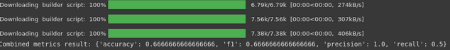
print(f"Combined metrics result: {results}")

Output:

Explanation:

1. evaluate.combine takes a list of metric names and returns a combined evaluation object.
2. Calling compute on this object calculates all the specified metrics using the same input data.

Using Measurements

Measurements can be used to analyze datasets. Here’s how to use the word_length measurement:

import evaluate

# Load the word_length measurement

# Note: May require NLTK data download on first run

try:

   word_length = evaluate.load("word_length", module_type="measurement")

   data = ["hello world", "this is another sentence"]

   results = word_length.compute(data=data)

   print(f"Word length measurement result: {results}")

except Exception as e:

   print(f"Could not run word_length measurement, possibly NLTK data missing: {e}")

   print("Attempting NLTK download...")

   import nltk

   nltk.download('punkt') # Uncomment and run if needed

Output:

Explanation:

1. We load word_length and specify module_type=”measurement”.
2. The compute method takes the dataset (a list of strings here) as input.
3. It returns statistics about the word lengths in the provided data. (Note: Requires nltk and its ‘punkt’ tokenizer data).

Evaluating Specific NLP Tasks

Different NLP tasks require specific metrics. Hugging Face Evaluate includes many standard ones.

Machine Translation (BLEU)

BLEU (Bilingual Evaluation Understudy) is common for translation quality. It measures n-gram overlap between the model’s translation (hypothesis) and reference translations.

import evaluate

def evaluate_machine_translation(hypotheses, references):

   """Calculates BLEU score for machine translation."""

   bleu_metric = evaluate.load("bleu")

   results = bleu_metric.compute(predictions=hypotheses, references=references)

   # Extract the main BLEU score

   bleu_score = results["bleu"]

   return bleu_score

# Example hypotheses (model translations)

hypotheses = ["the cat sat on mat.", "the dog played in garden."]

# Example references (correct translations, can have multiple per hypothesis)

references = [["the cat sat on the mat."], ["the dog played in the garden."]]

bleu_score = evaluate_machine_translation(hypotheses, references)

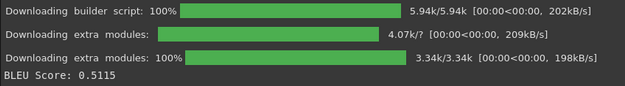
print(f"BLEU Score: {bleu_score:.4f}") # Format for readability

Output:

Explanation:

1. The function loads the BLEU metric.
2. It computes the score comparing predicted translations (hypotheses) against one or more correct references.
3. A higher BLEU score (closer to 1.0) generally indicates better translation quality, suggesting more overlap with reference translations. A score around 0.51 suggests moderate overlap.

Named Entity Recognition (NER – using seqeval)

For sequence labeling tasks like NER, metrics like precision, recall, and F1-score per entity type are useful. The seqeval metric handles this format (e.g., B-PER, I-PER, O tags).

To run the following code, seqeval library would be required. It could be installed by running the following command:

pip install seqeval

Code:

import evaluate

# Load the seqeval metric
try:

   seqeval_metric = evaluate.load("seqeval")

   # Example labels (using IOB format)
   true_labels = [['O', 'B-PER', 'I-PER', 'O'], ['B-LOC', 'I-LOC', 'O']]

   predicted_labels = [['O', 'B-PER', 'I-PER', 'O'], ['B-LOC', 'I-LOC', 'O']] # Example: Perfect prediction here

   results = seqeval_metric.compute(predictions=predicted_labels, references=true_labels)

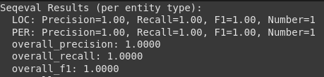
   print("Seqeval Results (per entity type):")

   # Print results nicely

   for key, value in results.items():

       if isinstance(value, dict):

           print(f"  {key}: Precision={value['precision']:.2f}, Recall={value['recall']:.2f}, F1={value['f1']:.2f}, Number={value['number']}")

       else:

           print(f"  {key}: {value:.4f}")

except ModuleNotFoundError:

   print("Seqeval metric not installed. Run: pip install seqeval")

Output:

Explanation:

• We load the seqeval metric.
• It takes lists of lists, where each inner list represents the tags for a sentence.
• The compute method returns detailed precision, recall, and F1 scores for each entity type identified (like PER for Person, LOC for Location) and overall scores.

Text Summarization (ROUGE)

ROUGE (Recall-Oriented Understudy for Gisting Evaluation) compares a generated summary against reference summaries, focusing on overlapping n-grams and longest common subsequences.

import evaluate

def simple_summarizer(text):

   """A very basic summarizer - just takes the first sentence."""

   try:

       sentences = text.split(".")

       return sentences[0].strip() + "." if sentences[0].strip() else ""

   except:

       return "" # Handle empty or malformed text

# Load ROUGE metric

rouge_metric = evaluate.load("rouge")

# Example text and reference summary

text = "Today is a beautiful day. The sun is shining and the birds are singing. I am going for a walk in the park."

reference = "The weather is pleasant today."

# Generate summary using the simple function

prediction = simple_summarizer(text)

print(f"Generated Summary: {prediction}")

print(f"Reference Summary: {reference}")

# Compute ROUGE scores

rouge_results = rouge_metric.compute(predictions=[prediction], references=[reference])

print(f"ROUGE Scores: {rouge_results}")

Output:

Generated Summary: Today is a beautiful day.

Reference Summary: The weather is pleasant today.

ROUGE Scores: {'rouge1': np.float64(0.4000000000000001), 'rouge2':
 np.float64(0.0), 'rougeL': np.float64(0.20000000000000004), 'rougeLsum':
 np.float64(0.20000000000000004)}

Explanation:

1. We load the rouge metric.
2. We define a simplistic summarizer for demonstration.
3. compute calculates different ROUGE scores:
4. Scores closer to 1.0 indicate higher similarity to the reference summary. The low scores here reflect the basic nature of our simple_summarizer.

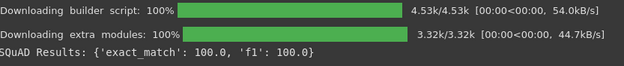
Question Answering (SQuAD)

The SQuAD metric is used for extractive question answering benchmarks. It calculates Exact Match (EM) and F1-score.

import evaluate

# Load the SQuAD metric

squad_metric = evaluate.load("squad")

# Example predictions and references format for SQuAD

predictions = [{'prediction_text': '1976', 'id': '56e10a3be3433e1400422b22'}]

references = [{'answers': {'answer_start': [97], 'text': ['1976']}, 'id': '56e10a3be3433e1400422b22'}]

results = squad_metric.compute(predictions=predictions, references=references)

print(f"SQuAD Results: {results}")

Output:

Explanation:

1. Loads the squad metric.
2. Takes predictions and references in a specific dictionary format, including the predicted text and the ground truth answers with their start positions.
3. exact_match: Percentage of predictions that exactly match one of the ground truth answers.
4. f1: Average F1 score over all questions, considering partial matches at the token level.

Advanced Evaluation with the Evaluator Class

The Evaluator class streamlines the process by integrating model loading, inference, and metric calculation. It’s particularly useful for standard tasks like text classification.

# Note: Requires transformers and datasets libraries
# pip install transformers datasets torch # or tensorflow/jax

import evaluate

from evaluate import evaluator

from transformers import pipeline

from datasets import load_dataset

# Load a pre-trained text classification pipeline
# Using a smaller model for potentially faster execution

try:

   pipe = pipeline("text-classification", model="distilbert-base-uncased-finetuned-sst-2-english", device=-1) # Use CPU

except Exception as e:

   print(f"Could not load pipeline: {e}")

   pipe = None

if pipe:

   # Load a small subset of the IMDB dataset

   try:

       data = load_dataset("imdb", split="test").shuffle(seed=42).select(range(100)) # Smaller subset for speed

   except Exception as e:

       print(f"Could not load dataset: {e}")

       data = None

   if data:

       # Load the accuracy metric

       accuracy_metric = evaluate.load("accuracy")

       # Create an evaluator for the task

       task_evaluator = evaluator("text-classification")

       # Correct label_mapping for IMDB dataset

       label_mapping = {

           'NEGATIVE': 0,  # Map NEGATIVE to 0

           'POSITIVE': 1   # Map POSITIVE to 1

       }

       # Compute results

       eval_results = task_evaluator.compute(

           model_or_pipeline=pipe,

           data=data,

           metric=accuracy_metric,

           input_column="text",  # Specify the text column

           label_column="label", # Specify the label column

           label_mapping=label_mapping  # Pass the corrected label mapping

       )

       print("\nEvaluator Results:")

       print(eval_results)

       # Compute with bootstrapping for confidence intervals

       bootstrap_results = task_evaluator.compute(

           model_or_pipeline=pipe,

           data=data,

           metric=accuracy_metric,

           input_column="text",

           label_column="label",

           label_mapping=label_mapping,  # Pass the corrected label mapping

           strategy="bootstrap",

           n_resamples=10  # Use fewer resamples for faster demo

       )

       print("\nEvaluator Results with Bootstrapping:")

       print(bootstrap_results)

Output:

Device set to use cpu

Evaluator Results:

{'accuracy': 0.9, 'total_time_in_seconds': 24.277618517999997,
'samples_per_second': 4.119020155368932, 'latency_in_seconds':
0.24277618517999996}

Evaluator Results with Bootstrapping:

{'accuracy': {'confidence_interval': (np.float64(0.8703044820750653),
np.float64(0.9335706530476571)), 'standard_error':
np.float64(0.02412928142780514), 'score': 0.9}, 'total_time_in_seconds':
23.871316319000016, 'samples_per_second': 4.189128017226537,
'latency_in_seconds': 0.23871316319000013}

Explanation:

1. We load a transformers pipeline for text classification and a sample of the IMDb dataset.
2. We create an evaluator specifically for “text-classification”.
3. The compute method handles feeding data (text column) to the pipeline, getting predictions, comparing them to the true labels (label column) using the specified metric, and applying the label_mapping.
4. It returns the metric score along with performance stats like total time and samples per second.
5. Using strategy=”bootstrap” performs resampling to estimate confidence intervals and standard error for the metric, giving a sense of the score’s stability.

Using Evaluation Suites

Evaluation Suites bundle multiple evaluations, often targeting specific benchmarks like GLUE. This allows running a model against a standard set of tasks.

# Note: Running a full suite can be computationally intensive and time-consuming.

# This example demonstrates the concept but might take a long time or require significant resources.

# It also installs multiple datasets and may require specific model configurations.

import evaluate

try:

   print("\nLoading GLUE evaluation suite (this might download datasets)...")

   # Load the GLUE task directly

   # Using "mrpc" as an example task, but you can choose from the valid ones listed above

   task = evaluate.load("glue", "mrpc")  # Specify the task like "mrpc", "sst2", etc.

   print("Task loaded.")

   # You can now run the task on a model (for example: "distilbert-base-uncased")

   # WARNING: This might take time for inference or fine-tuning.

   # results = task.compute(model_or_pipeline="distilbert-base-uncased")

   # print("\nEvaluation Results (MRPC Task):")

   # print(results)

   print("Skipping model inference for brevity in this example.")

   print("Refer to Hugging Face documentation for full EvaluationSuite usage.")

except Exception as e:

   print(f"Could not load or run evaluation suite: {e}")

Output:

Loading GLUE evaluation suite (this might download datasets)...

Task loaded.

Skipping model inference for brevity in this example.

Refer to Hugging Face documentation for full EvaluationSuite usage.

Explanation:

1. EvaluationSuite.load loads a predefined set of evaluation tasks (here, just the MRPC task from the GLUE benchmark for demonstration).
2. The suite.run(“model_name”) command would typically execute the model on each dataset within the suite and compute the relevant metrics.
3. The output is usually a list of dictionaries, each containing the results for one task in the suite. (Note: Running this often requires specific environment setups and substantial compute time).

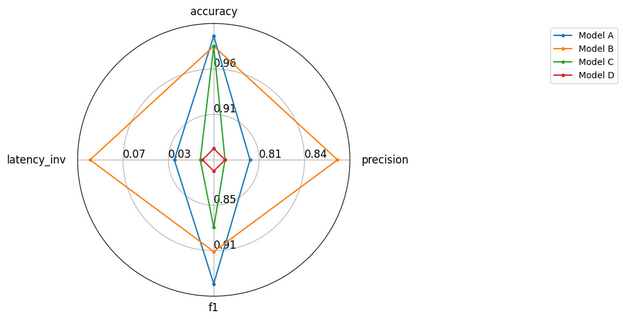
Visualizing Evaluation Results

Visualizations help compare multiple models across different metrics. Radar plots are effective for this.

import evaluate

import matplotlib.pyplot as plt # Ensure matplotlib is installed

from evaluate.visualization import radar_plot

# Sample data for multiple models across several metrics

# Lower latency is better, so we might invert it or consider it separately.

data = [

   {"accuracy": 0.99, "precision": 0.80, "f1": 0.95, "latency_inv": 1/33.6},

   {"accuracy": 0.98, "precision": 0.87, "f1": 0.91, "latency_inv": 1/11.2},

   {"accuracy": 0.98, "precision": 0.78, "f1": 0.88, "latency_inv": 1/87.6},

   {"accuracy": 0.88, "precision": 0.78, "f1": 0.81, "latency_inv": 1/101.6}

]

model_names = ["Model A", "Model B", "Model C", "Model D"]

# Generate the radar plot

# Higher values are generally better on a radar plot

try:

   # Generate radar plot (ensure you pass a correct format and that data is valid)

   plot = radar_plot(data=data, model_names=model_names)

   # Display the plot

   plt.show()  # Explicitly show the plot, might be necessary in some environments

   # To save the plot to a file (uncomment to use)

   # plot.savefig("model_comparison_radar.png")

   plt.close() # Close the plot window after showing/saving

except ImportError:

   print("Visualization requires matplotlib. Run: pip install matplotlib")

except Exception as e:

   print(f"Could not generate plot: {e}")

Output:

Explanation:

1. We prepare sample results for four models across accuracy, precision, F1, and inverted latency (so higher is better).
2. radar_plot creates a plot where each axis represents a metric, showing how models compare visually.

Saving Evaluation Results

You can save your evaluation results to a file, often in JSON format, for record-keeping or later analysis.

import evaluate

from pathlib import Path

# Perform an evaluation

accuracy_metric = evaluate.load("accuracy")

result = accuracy_metric.compute(references=[0, 1, 0, 1], predictions=[1, 0, 0, 1])

print(f"Result to save: {result}")

# Define hyperparameters or other metadata

hyperparams = {"model_name": "my_custom_model", "learning_rate": 0.001}

run_details = {"experiment_id": "run_42"}

# Combine results and metadata

save_data = {**result, **hyperparams, **run_details}

# Define save directory and filename

save_dir = Path("./evaluation_results")

save_dir.mkdir(exist_ok=True) # Create directory if it doesn't exist

# Use evaluate.save to store the results

try:

   saved_path = evaluate.save(save_directory=save_dir, **save_data)

   print(f"Results saved to: {saved_path}")

   # You can also manually save as JSON

   import json

   manual_save_path = save_dir / "manual_results.json"

   with open(manual_save_path, 'w') as f:

       json.dump(save_data, f, indent=4)

   print(f"Results manually saved to: {manual_save_path}")

except Exception as e:

    # Catch potential git-related errors if run outside a repo

    print(f"evaluate.save encountered an issue (possibly git related): {e}")

    print("Attempting manual JSON save instead.")

    import json

    manual_save_path = save_dir / "manual_results_fallback.json"

    with open(manual_save_path, 'w') as f:

        json.dump(save_data, f, indent=4)

    print(f"Results manually saved to: {manual_save_path}")

Output:

Result to save: {'accuracy': 0.5}

evaluate.save encountered an issue (possibly git related): save() missing 1
 required positional argument: 'path_or_file'

Attempting manual JSON save instead.

Results manually saved to: evaluation_results/manual_results_fallback.json

Explanation:

1. We combine the computed result dictionary with other metadata like hyperparams.
2. evaluate.save attempts to save this data to a JSON file in the specified directory. It might try to add git commit information if run within a repository, which can cause errors otherwise (as seen in the original log).
3. We include a fallback to manually save the dictionary as a JSON file, which is often sufficient.

Choosing the Right Metric

Selecting the appropriate metric is crucial. Consider these points:

1. Task Type: Is it classification, translation, summarization, NER, QA? Use metrics standard for that task (Accuracy/F1 for classification, BLEU/ROUGE for generation, Seqeval for NER, SQuAD for QA).
2. Dataset: Some benchmarks (like GLUE, SQuAD) have specific associated metrics. Leaderboards (e.g., on Papers With Code) often show commonly used metrics for specific datasets.
3. Goal: What aspect of performance matters most?
   • Accuracy: Overall correctness (good for balanced classes).
   • Precision/Recall/F1: Important for imbalanced classes or when false positives/negatives have different costs.
   • BLEU/ROUGE: Fluency and content overlap in text generation.
   • Perplexity: How well a language model predicts a sample (lower is better, often used for generative models).
4. Metric Cards: Read the Hugging Face metric cards (documentation) for detailed explanations, limitations, and appropriate use cases (e.g., BLEU card, SQuAD card).

Conclusion

The Hugging Face Evaluate library offers a versatile and user-friendly way to assess large language models and datasets. It provides standard metrics, dataset measurements, and tools like the Evaluator and EvaluationSuite to streamline the process. By using these tools and choosing metrics appropriate for your task, you can gain clear insights into your model’s strengths and weaknesses.

For more details and advanced usage, consult the official resources:

• Hugging Face Evaluate Documentation: Quick Tour
• GitHub Repository: huggingface/evaluate
• Kaggle Notebook Example: LLM Evaluation Framework (Source of some examples used here)

Harsh Mishra

Harsh Mishra is an AI/ML Engineer who spends more time talking to Large Language Models than actual humans. Passionate about GenAI, NLP, and making machines smarter (so they don’t replace him just yet). When not optimizing models, he’s probably optimizing his coffee intake. 🚀☕